Example input data sets
Details
exidataholds individual-level parameters and other data items, one per rowextran1is a "condensed" data setextran2is a full datasetextran3is a full dataset with parametersexTheophis the theophylline data set, ready for input intomrgsolveexBoota set of bootstrap parameter estimates
Examples
mod <- mrgsolve::house() %>% update(end=240) %>% Req(CP)
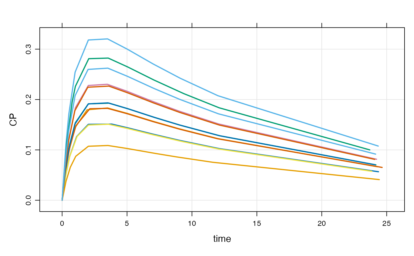
## Full data set
data(exTheoph)
out <- mod %>% data_set(exTheoph) %>% mrgsim
out
#> Model: housemodel
#> Dim: 132 x 3
#> Time: 0 to 24.65
#> ID: 12
#> ID time CP
#> 1: 1 0.00 0.00000
#> 2: 1 0.25 0.04552
#> 3: 1 0.57 0.08624
#> 4: 1 1.12 0.12643
#> 5: 1 2.02 0.15072
#> 6: 1 3.82 0.15121
#> 7: 1 5.10 0.14348
#> 8: 1 7.03 0.13101
plot(out)
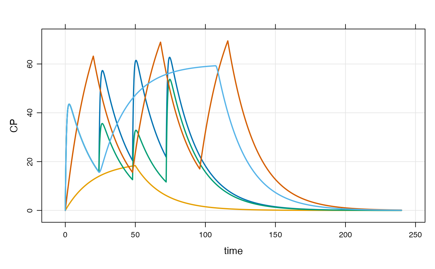
 ## Condensed: mrgsolve fills in the observations
data(extran1)
out <- mod %>% data_set(extran1) %>% mrgsim
out
#> Model: housemodel
#> Dim: 4814 x 3
#> Time: 0 to 240
#> ID: 5
#> ID time CP
#> 1: 1 0.00 0.00
#> 2: 1 0.00 0.00
#> 3: 1 0.25 12.87
#> 4: 1 0.50 22.25
#> 5: 1 0.75 29.04
#> 6: 1 1.00 33.91
#> 7: 1 1.25 37.37
#> 8: 1 1.50 39.78
plot(out)
## Condensed: mrgsolve fills in the observations
data(extran1)
out <- mod %>% data_set(extran1) %>% mrgsim
out
#> Model: housemodel
#> Dim: 4814 x 3
#> Time: 0 to 240
#> ID: 5
#> ID time CP
#> 1: 1 0.00 0.00
#> 2: 1 0.00 0.00
#> 3: 1 0.25 12.87
#> 4: 1 0.50 22.25
#> 5: 1 0.75 29.04
#> 6: 1 1.00 33.91
#> 7: 1 1.25 37.37
#> 8: 1 1.50 39.78
plot(out)
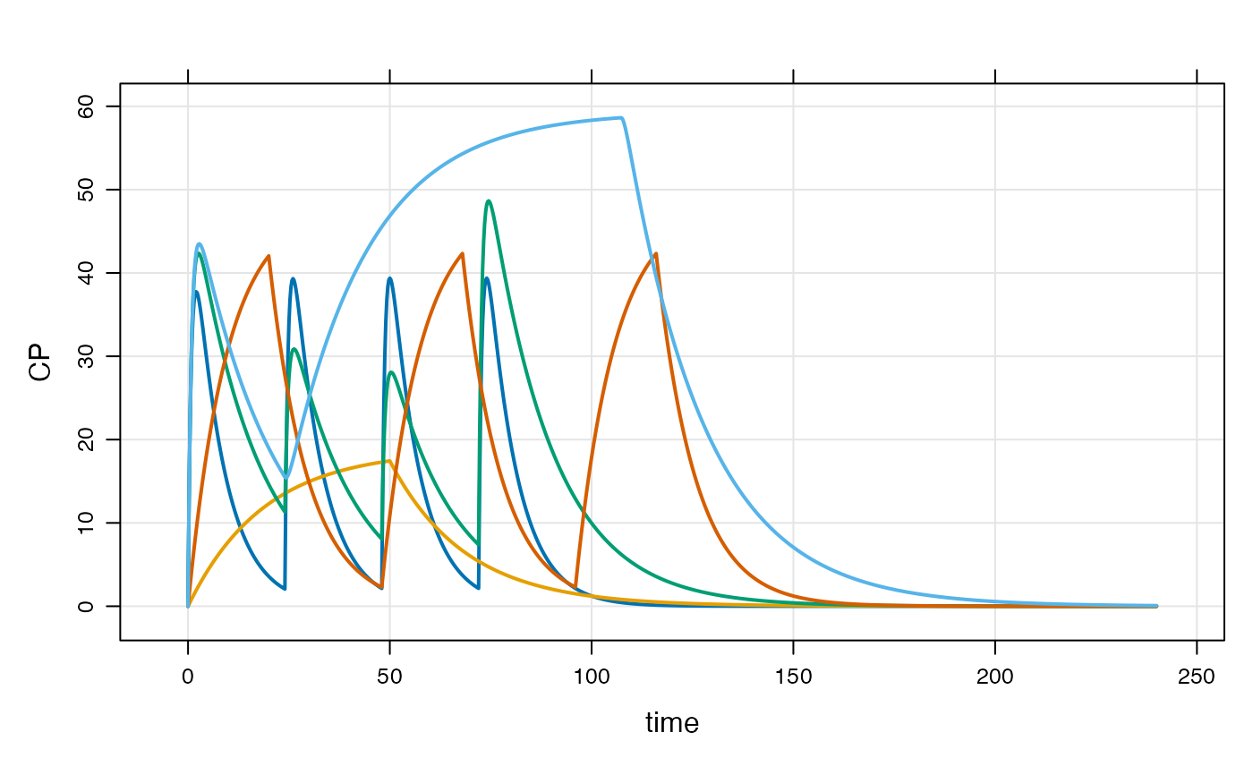
 ## Add a parameter to the data set
stopifnot(require(dplyr))
#> Loading required package: dplyr
#>
#> Attaching package: ‘dplyr’
#> The following objects are masked from ‘package:stats’:
#>
#> filter, lag
#> The following objects are masked from ‘package:base’:
#>
#> intersect, setdiff, setequal, union
data <- extran1 %>% distinct(ID) %>% select(ID) %>%
mutate(CL=exp(log(1.5) + rnorm(nrow(.), 0,sqrt(0.1)))) %>%
left_join(extran1,.)
#> Joining with `by = join_by(ID)`
data
#> ID amt cmt time addl ii rate evid CL
#> 1 1 1000 1 0 3 24 0 1 2.353306
#> 2 2 1000 2 0 0 0 20 1 2.200713
#> 3 3 1000 1 0 0 0 0 1 1.668183
#> 4 3 500 1 24 0 0 0 1 1.668183
#> 5 3 500 1 48 0 0 0 1 1.668183
#> 6 3 1000 1 72 0 0 0 1 1.668183
#> 7 4 2000 2 0 2 48 100 1 1.891836
#> 8 5 1000 1 0 0 0 0 1 1.212548
#> 9 5 5000 1 24 0 0 60 1 1.212548
out <- mod %>% data_set(data) %>% carry_out(CL) %>% mrgsim
out
#> Model: housemodel
#> Dim: 4814 x 4
#> Time: 0 to 240
#> ID: 5
#> ID time CL CP
#> 1: 1 0.00 2.353 0.00
#> 2: 1 0.00 2.353 0.00
#> 3: 1 0.25 2.353 12.76
#> 4: 1 0.50 2.353 21.84
#> 5: 1 0.75 2.353 28.21
#> 6: 1 1.00 2.353 32.59
#> 7: 1 1.25 2.353 35.48
#> 8: 1 1.50 2.353 37.30
plot(out)
## Add a parameter to the data set
stopifnot(require(dplyr))
#> Loading required package: dplyr
#>
#> Attaching package: ‘dplyr’
#> The following objects are masked from ‘package:stats’:
#>
#> filter, lag
#> The following objects are masked from ‘package:base’:
#>
#> intersect, setdiff, setequal, union
data <- extran1 %>% distinct(ID) %>% select(ID) %>%
mutate(CL=exp(log(1.5) + rnorm(nrow(.), 0,sqrt(0.1)))) %>%
left_join(extran1,.)
#> Joining with `by = join_by(ID)`
data
#> ID amt cmt time addl ii rate evid CL
#> 1 1 1000 1 0 3 24 0 1 2.353306
#> 2 2 1000 2 0 0 0 20 1 2.200713
#> 3 3 1000 1 0 0 0 0 1 1.668183
#> 4 3 500 1 24 0 0 0 1 1.668183
#> 5 3 500 1 48 0 0 0 1 1.668183
#> 6 3 1000 1 72 0 0 0 1 1.668183
#> 7 4 2000 2 0 2 48 100 1 1.891836
#> 8 5 1000 1 0 0 0 0 1 1.212548
#> 9 5 5000 1 24 0 0 60 1 1.212548
out <- mod %>% data_set(data) %>% carry_out(CL) %>% mrgsim
out
#> Model: housemodel
#> Dim: 4814 x 4
#> Time: 0 to 240
#> ID: 5
#> ID time CL CP
#> 1: 1 0.00 2.353 0.00
#> 2: 1 0.00 2.353 0.00
#> 3: 1 0.25 2.353 12.76
#> 4: 1 0.50 2.353 21.84
#> 5: 1 0.75 2.353 28.21
#> 6: 1 1.00 2.353 32.59
#> 7: 1 1.25 2.353 35.48
#> 8: 1 1.50 2.353 37.30
plot(out)
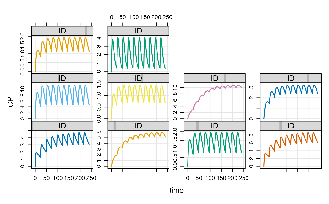
 ## idata
data(exidata)
out <- mod %>% idata_set(exidata) %>% ev(amt=100,ii=24,addl=10) %>% mrgsim
plot(out, CP~time|ID)
## idata
data(exidata)
out <- mod %>% idata_set(exidata) %>% ev(amt=100,ii=24,addl=10) %>% mrgsim
plot(out, CP~time|ID)