Methods for working with mrgsims objects

These methods help the user view simulation output and extract simulated data to work with further. The methods listed here for the most part have generics defined by R or other R packages. See the See Also section for other methods defined by mrgsolve that have their own documentation pages.

Usage

# S4 method for class 'mrgsims'
x$name

# S4 method for class 'mrgsims'
tail(x, ...)

# S4 method for class 'mrgsims'
head(x, ...)

# S4 method for class 'mrgsims'
dim(x)

# S4 method for class 'mrgsims'
names(x)

# S4 method for class 'mrgsims'
as.data.frame(x, row.names = NULL, optional = FALSE, ...)

# S4 method for class 'mrgsims'
as.matrix(x, ...)

# S3 method for class 'mrgsims'
summary(object, ...)

# S4 method for class 'mrgsims'
show(object)

Arguments

x

mrgsims object.

name

name of column of simulated output to retain

...

passed to other functions.

row.names

passed to as.data.frame().

optional

passed to as.data.frame().

object

passed to show.

Details

Most methods should behave as expected according to other method commonly used in R (e.g. head, tail, as.data.frame, etc ...)

• $ selects a column in the simulated data and returns numeric

• head() see head.matrix(); returns simulated data

• tail() see tail.matrix(); returns simulated data

• dim(), nrow(), ncol() returns dimensions, number of rows, and number of columns in simulated data

• as.data.frame() coerces simulated data to data.frame

• as.matrix() returns matrix of simulated data

• summary() coerces simulated data to data.frame and passes to summary.data.frame()

• plot() plots simulated data; see plot_mrgsims

See also

stime()

Examples

## example("mrgsims")

mod <- mrgsolve::house() %>% init(GUT=100)

out <- mrgsim(mod)

class(out)
#> [1] "mrgsims"
#> attr(,"package")
#> [1] "mrgsolve"

if (FALSE) { # \dontrun{
out
} # }
head(out)
#>   ID time       GUT     CENT     RESP       DV       CP
#> 1  1 0.00 100.00000  0.00000 50.00000 0.000000 0.000000
#> 2  1 0.25  74.08182 25.74883 48.68223 1.287441 1.287441
#> 3  1 0.50  54.88116 44.50417 46.18005 2.225208 2.225208
#> 4  1 0.75  40.65697 58.08258 43.61333 2.904129 2.904129
#> 5  1 1.00  30.11942 67.82976 41.37943 3.391488 3.391488
#> 6  1 1.25  22.31302 74.74256 39.57649 3.737128 3.737128
tail(out)
#>     ID   time          GUT      CENT     RESP         DV         CP
#> 476  1 118.75 9.263629e-44 0.2753340 49.92950 0.01376670 0.01376670
#> 477  1 119.00 5.404491e-44 0.2719137 49.93038 0.01359569 0.01359569
#> 478  1 119.25 2.473491e-44 0.2685360 49.93124 0.01342680 0.01342680
#> 479  1 119.50 2.514809e-44 0.2652002 49.93209 0.01326001 0.01326001
#> 480  1 119.75 1.885697e-44 0.2619058 49.93293 0.01309529 0.01309529
#> 481  1 120.00 1.174272e-44 0.2586523 49.93377 0.01293262 0.01293262


dim(out)
#> [1] 481   7
names(out)
#> [1] "ID"   "time" "GUT"  "CENT" "RESP" "DV"   "CP"  

mat <- as.matrix(out)
df <- as.data.frame(out)

if (FALSE) { # \dontrun{
out$CP
} # }

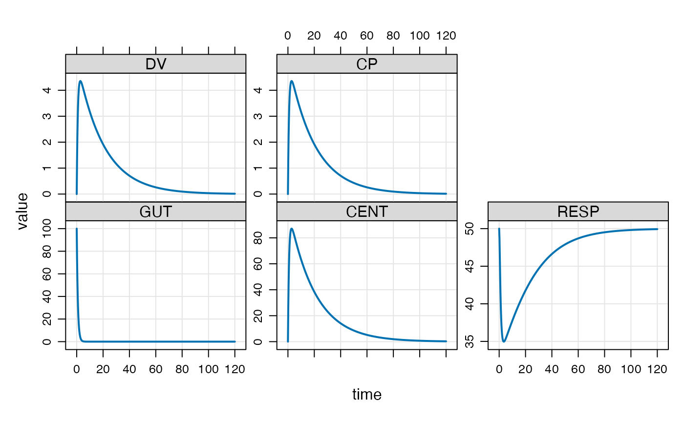
plot(out)


if (FALSE) { # \dontrun{
plot(out, CP~.)
plot(out, CP+RESP~time, scales="same", xlab="Time", main="Model sims")
} # }