8  Dose by dose regimen

Previous vignettes showed how to schedule a series of doses into the future. This vignette shows a dosing regimen that proceds dose-by-dose. This approach is the gateway to doing highly-customized adaptive dosing.

In this example, we dose by infusion.

• Use the evtools plugin
• The dynamic dosing stuff goes in the [ event ] block
• Whenever TIME matches up with the expected dosing time (based on INTERVAL), we trigger a dose.
• Then push() the object back to mrgsolve

8.1 Check next dose using std::fmod()

model/evtools-3.solv

[ plugin ] evtools

[ set ] outvars = "CP"

[ param ] 

CL = 1
V = 32
KA = 2

DOSE = 100
INTERVAL = 24
OVER = 2

[ pkmodel ] advan = 2

[ event ] 

if(std::fmod(TIME, INTERVAL) == 0) {
  evt::infuse(self, DOSE, 2, DOSE/OVER); 
}

[ error ] capture CP = A2/V;

mod <- mread("model/evtools-3.solv")

. Building evtools-3_solv ... done.

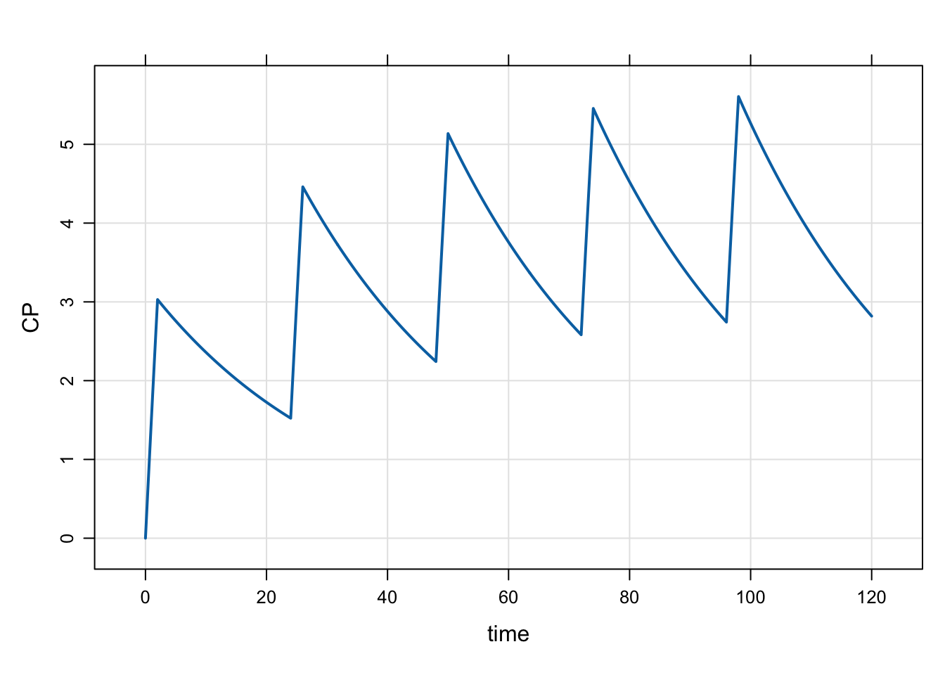
out <- mrgsim(mod, end = 120, delta = 0.25)

plot(out)

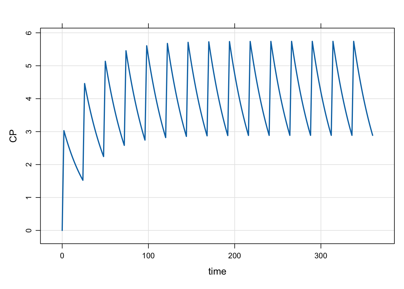
We didn’t really specify a dose end time, so the dosing will go as long as we simulate.

out <- mrgsim(mod, end = 360, delta = 0.25)

plot(out)

8.2 Check next dose using evt::near()

In model 4, we have a slightly different mechanism for figuring out when the next dose should be given - using the evt::near() function.

model/evtools-4.solv

[ plugin ] evtools

[ set ] outvars = "CP"

[ param ] 

CL = 1
V = 32
KA = 2

DOSE = 100
INTERVAL = 24
OVER = 2
END = 240

[ pkmodel ]

cmt = "A1,A2"
depot = TRUE

[ event ] 

if(TIME > END) return;

if(NEWIND <=1) { 
  double nextdose = 0;
}

if(evt::near(TIME, nextdose)) {
  evt::infuse(self, DOSE, 1, DOSE/OVER); 
  nextdose = nextdose + INTERVAL;
}

[ error ] 

capture CP = A2/V;

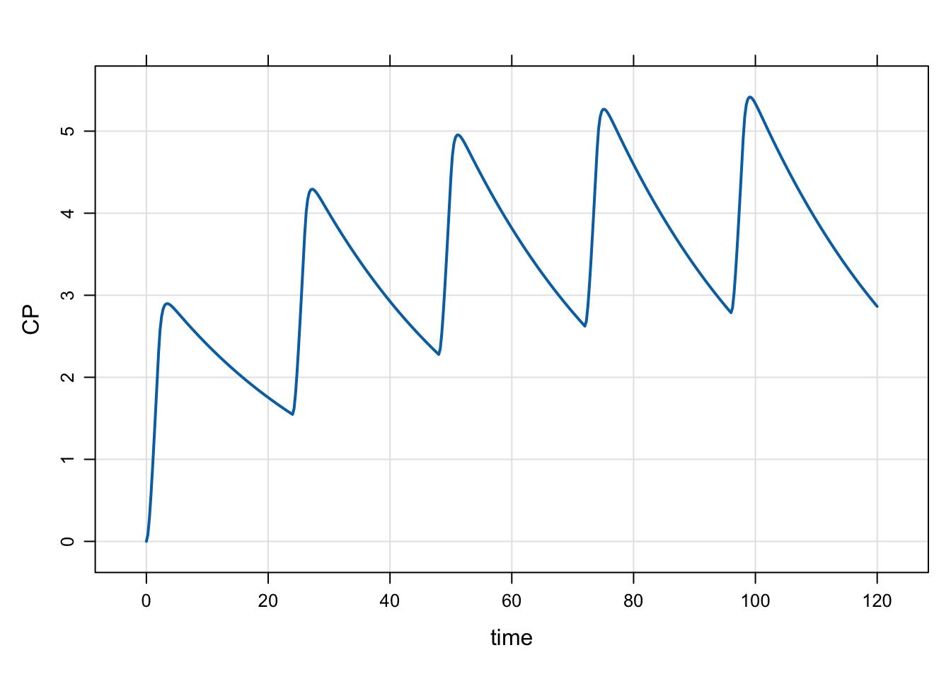
The mechanics should work the same as model 3.

mod <- mread("model/evtools-4.solv")

. Building evtools-4_solv ... done.

out <- mrgsim(mod, end = 120, delta = 0.25)

plot(out)