I just discovered this nifty tool published by the folks over at Occams (with other contributors as well) called pmxTools. There are a lot of really useful R functions for your pharmacometrics workflow in this package and worth checking it out in depth!

What I want to focus on for this post is how we can use this package to cross validate mrgsolve output: we’ll simulate with pmxTools and mrgsolve just to see the different workflows and check the output values. If users are interested in other validation tests for mrgsolve, please see the document here. This is not a “lets-go-head-to-head with another project” type post. I just found this tool very useful as a complement to my workflow. I hope you find it useful too.

1 Setup

library(mrgsolve)
library(dplyr)
library(ggplot2)
theme_set(theme_bw())
options(mrgsolve.soloc="build")

library(pmxTools)

Loading required package: MASS


Attaching package: 'MASS'

The following object is masked from 'package:dplyr':

    select

Loading required package: stringr

Loading required package: magrittr

Loading required package: data.tree

Loading required package: DiagrammeR


Attaching package: 'pmxTools'

The following object is masked from 'package:mrgsolve':

    read_nmext

2 Two-compartment infusion

2.1 Simulate with `pmxTools::pk_curve`

You can use this function to generate a PK profile based on super-positioning.

To simulate a 2-compartment model after IV infusion of 100 mg over 10 hours, first define a list of pk parameters, including tinf, the infusion duration

pars <- list(CL = 1, V1 = 4, V2 = 50, Q = 5, tinf=10)

Call pk_curve and provide simulation times, dose regimen (including dose, ii, addl), the model parameters, and select the model, in this case it is 2cmt_infusion

calc <- pk_curve(
  t = seq(0,400,0.1), 
  dose = 100, 
  ii = 24, 
  addl = 9, 
  params = pars, 
  model="2cmt_infusion"
)

head(calc)

    t        cp
1 0.0 0.0000000
2 0.1 0.2322016
3 0.2 0.4323273
4 0.3 0.6050735
5 0.4 0.7544486
6 0.5 0.8838735

ggplot(data = calc, aes(t,cp)) + geom_line() + theme_bw()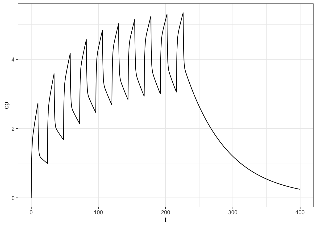

Pretty easy!

2.2 Simulate with mrgsolve

We can load the 2-compartment model from our model library, and update the parameter set. We make an event object with the dosing information and simulate:

mod <- 
  modlib("pk2", delta = 0.1, end = 400) %>% 
  param(CL = 1, V2 = 4, V3 = 50, Q = 5)

Loading model from cache.

e <- ev(amt = 100, rate = 10, ii = 24, addl = 9, cmt = 2)

out <- mrgsim_e(mod,e, obsonly=TRUE, recsort=3)

plot(out, CP~time)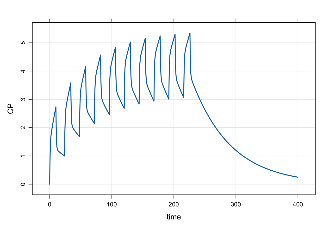

head(out)

  ID time EV      CENT     PERIPH        CP
1  1  0.0  0 0.0000000 0.00000000 0.0000000
2  1  0.1  0 0.9288064 0.05929462 0.2322016
3  1  0.2  0 1.7293093 0.22531873 0.4323273
4  1  0.3  0 2.4202941 0.48225334 0.6050735
5  1  0.4  0 3.0177942 0.81659743 0.7544486
6  1  0.5  0 3.5354939 1.21682828 0.8838735

2.3 Are they the same?

We can check the difference between the values:

summary(out$CP-calc[["cp"]])

      Min.    1st Qu.     Median       Mean    3rd Qu.       Max. 
-7.550e-14 -2.487e-14 -1.021e-14  2.443e-15  4.091e-14  5.751e-14

3 Oral dosing example

To do a model for first-order absorption

pars <- list(CL = 1, V = 20, ka = 1.2)

calc <- pk_curve(
  t = seq(0,400,0.1), 
  dose = 100, 
  ii = 24, 
  addl = 9, 
  params = pars, 
  model = "1cmt_oral"
)

ggplot(calc, aes(t,cp)) + geom_line() + theme_bw()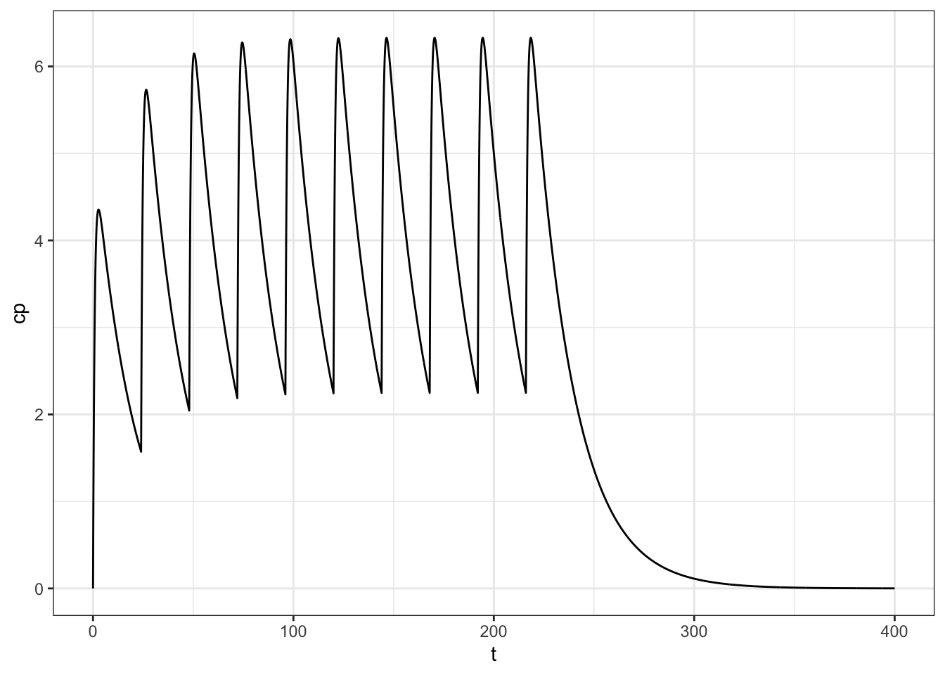

mod <- modlib("pk1", param = list(CL=1, V = 20, KA = 1.2), end=400, delta=0.1)

Loading model from cache.

out <- mrgsim_e(
  mod, 
  mutate(e, rate = 0, cmt = 1),
  recsort = 3, 
  obsonly = TRUE
)

plot(out, CP~time)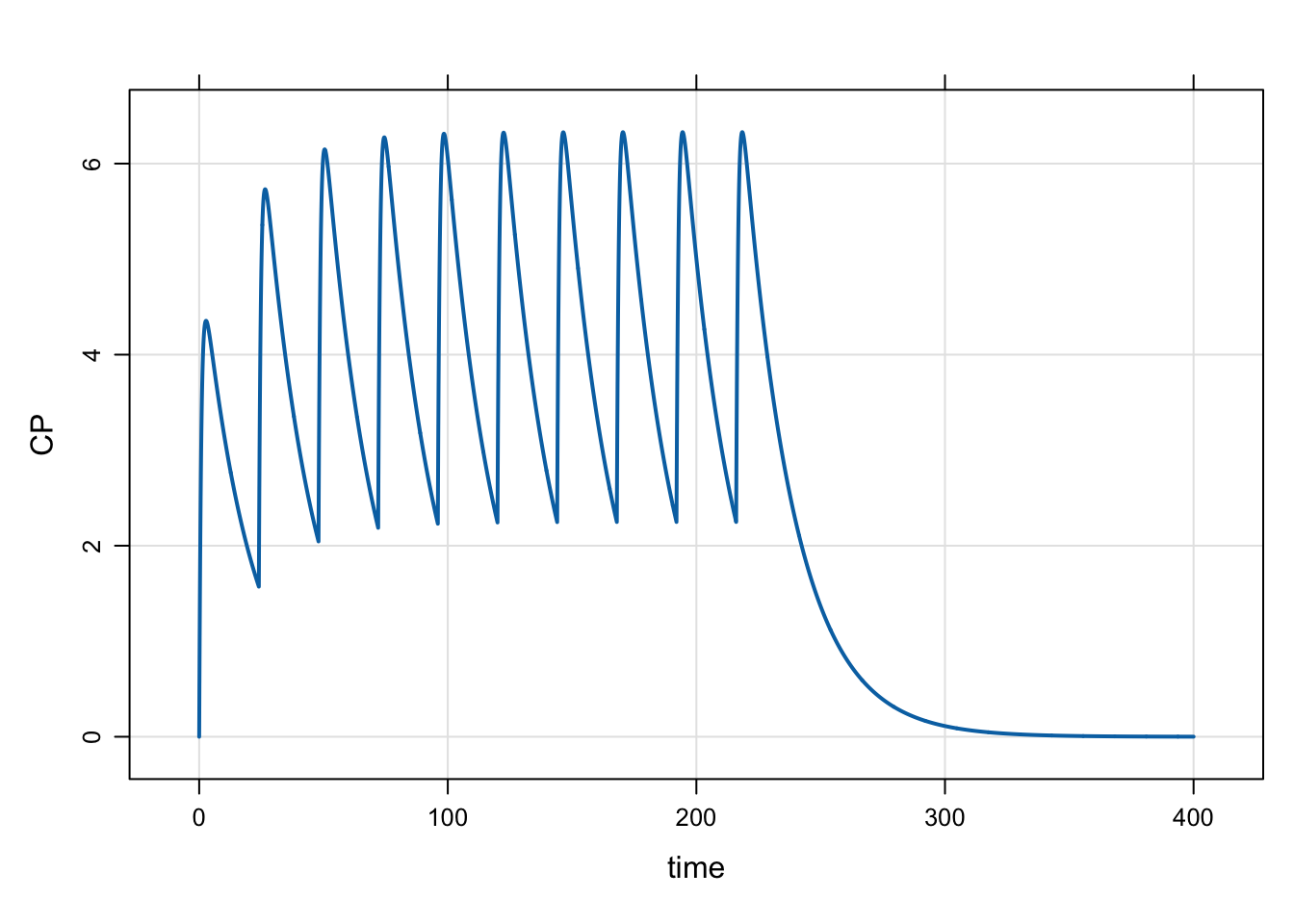

summary(out$CP-calc[["cp"]])

      Min.    1st Qu.     Median       Mean    3rd Qu.       Max. 
-5.640e-14 -3.286e-14 -1.998e-14 -1.767e-14 -4.233e-16  9.059e-14

4 Caution

Please note that we used some specific options to get the results exactly comparable. It really does take a lot of care to ensure that the setup is exactly the same for both tools when doing comparisons like this. If you start benchmarking and the results don’t come out the same, please go back and double check your setup to make sure you haven’t made any assumptions about how each tool works.

5 Building our community

As I noted earlier, the goal of this post wasn’t to go head-to-head with pmxTools. Rather, I wanted to show how the mrgsolve project can take advantage of this great tool to help our development and validate what we’re doing. I can only hope that others also find mrgsolve as useful for their project, validation or other type of simulation work that needs to get done. This sort of synergy between development projects is only possible with an open-source community dedicated to open and public development projects and sharing of knowledge and tools. The more we do this in our pharmacometrics community, the more progress we’ll all make and our science will advance. And we will have done it together.