I worked an example for a SIR model to show people in the ecology field how they can use mrgsolve for their ODE-based models.

1 Write the SIR model

library(mrgsolve)
library(tidyverse)

model <- '
$PARAM B = 1/70, mu = 1/70, Beta = 400, gamma = 365/14

$INIT S = 1-0.001-0.9, I = 0.001, R = 0.9

$ODE
double N = S+I+R;
dxdt_S = B-Beta*S*I/N-mu*S;
dxdt_I = Beta*S*I/N-(mu+gamma)*I;
dxdt_R = gamma*I-mu*R;

$TABLE
double R0 = Beta/(mu+gamma);
'

2 Compile and load

mod <- mcode("sir", model,  end = 30, delta = 1/120)

Building sir ... done.

3 Simulate

mod %>% mrgsim() %>% plot(scales = "same")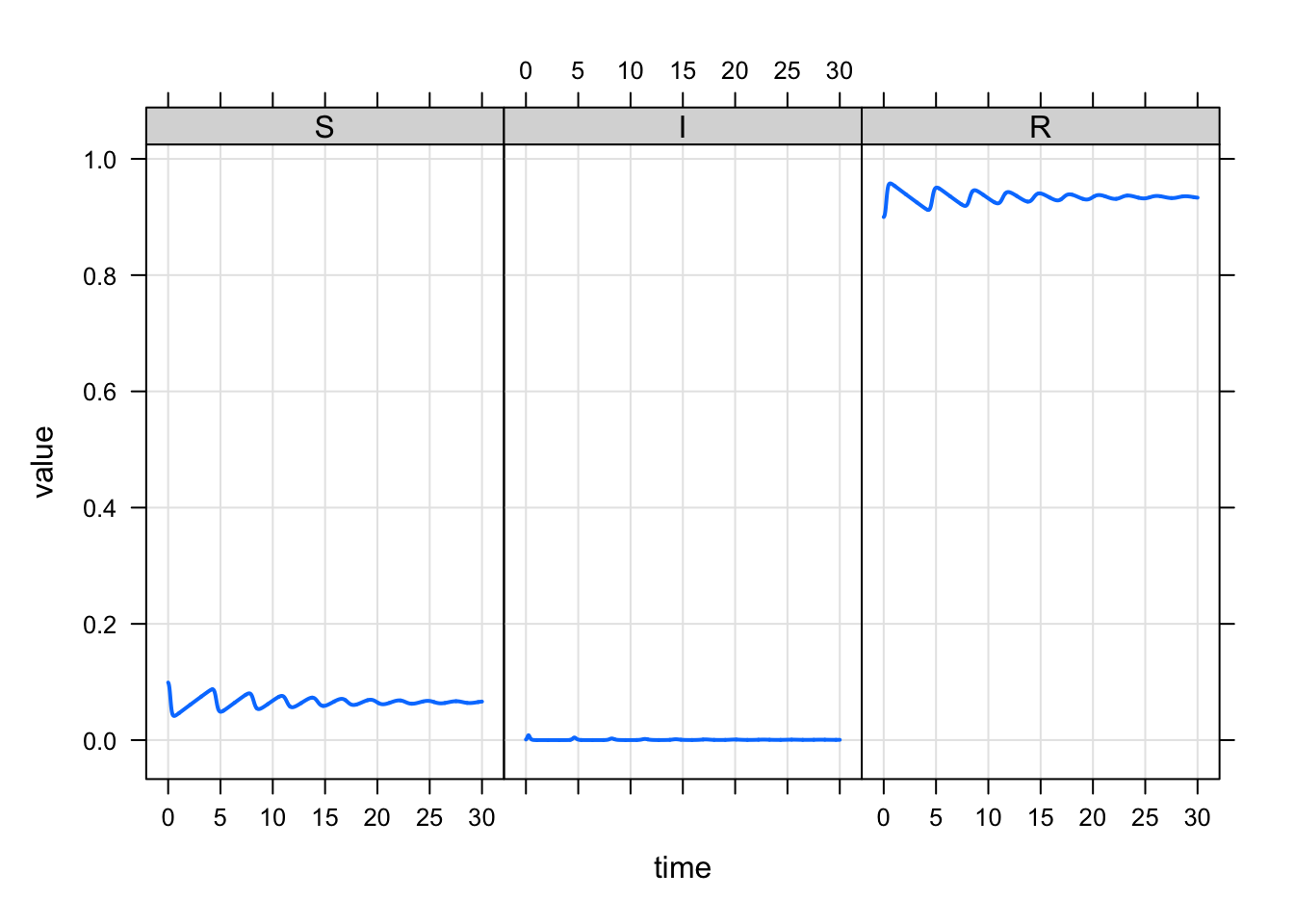

out <- mrgsim(mod, output="df")

ggplot(out, aes(S,I)) + geom_point()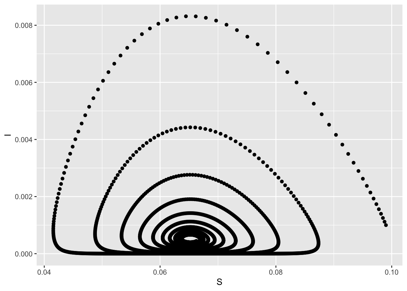

4 Challenge

Explore the dynamics of the system for different values of the beta and b parameters by simulating and plotting trajectories as time series and in phase space (e.g., I vs. S). How the beta, B, and R0 related to the type of trajectories you get?

mod %>%
  wf_sweep(Beta, cv = 10) %>%
  plot(R~time)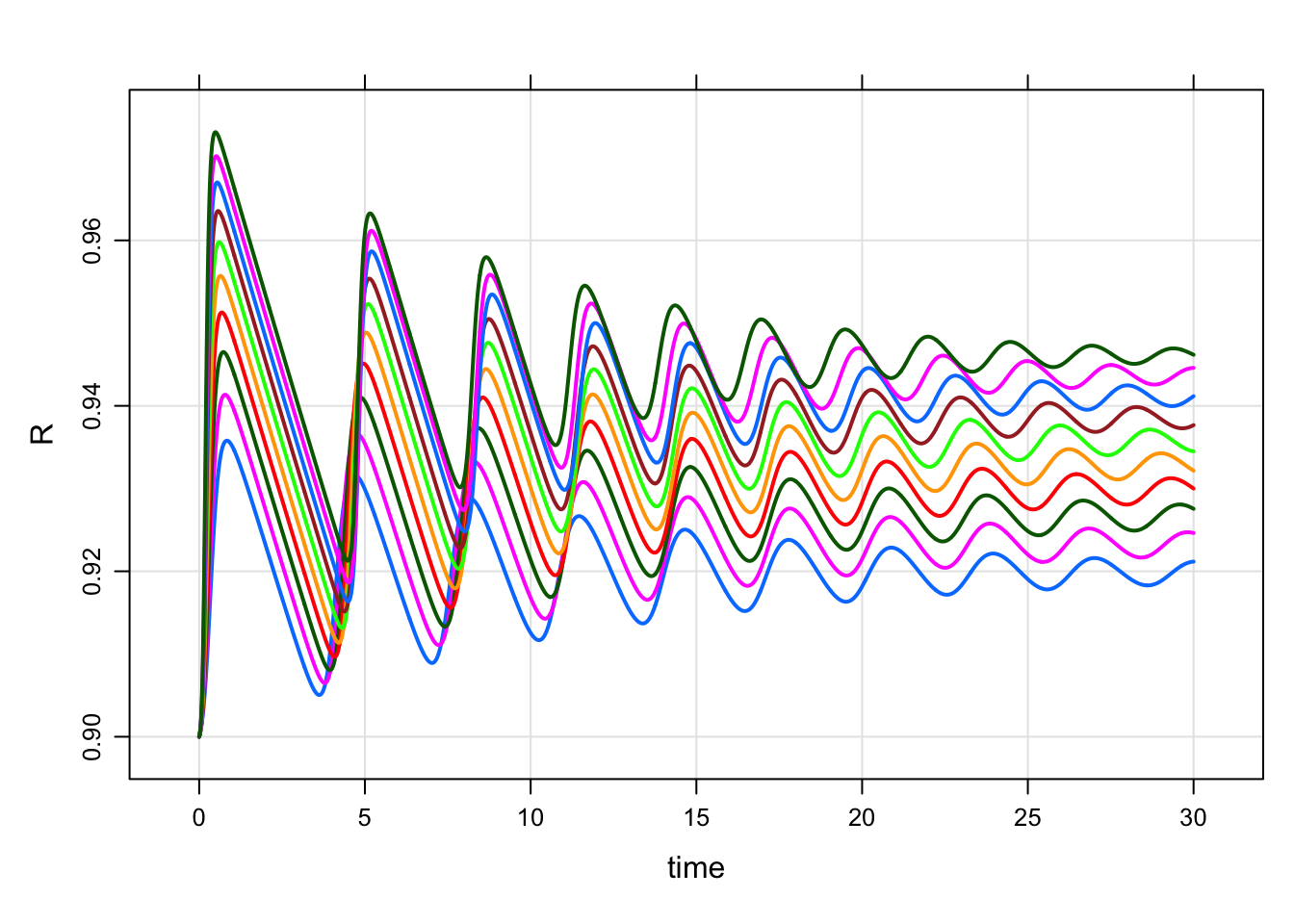

mod %>%
  wf_sweep(B, cv = 10) %>%
  plot(R~time)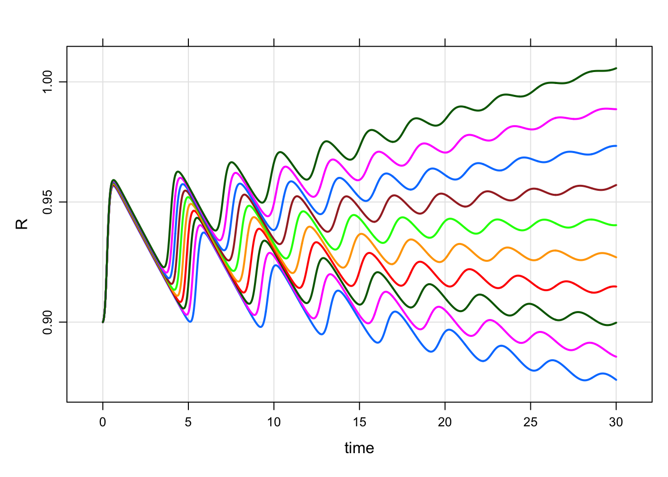

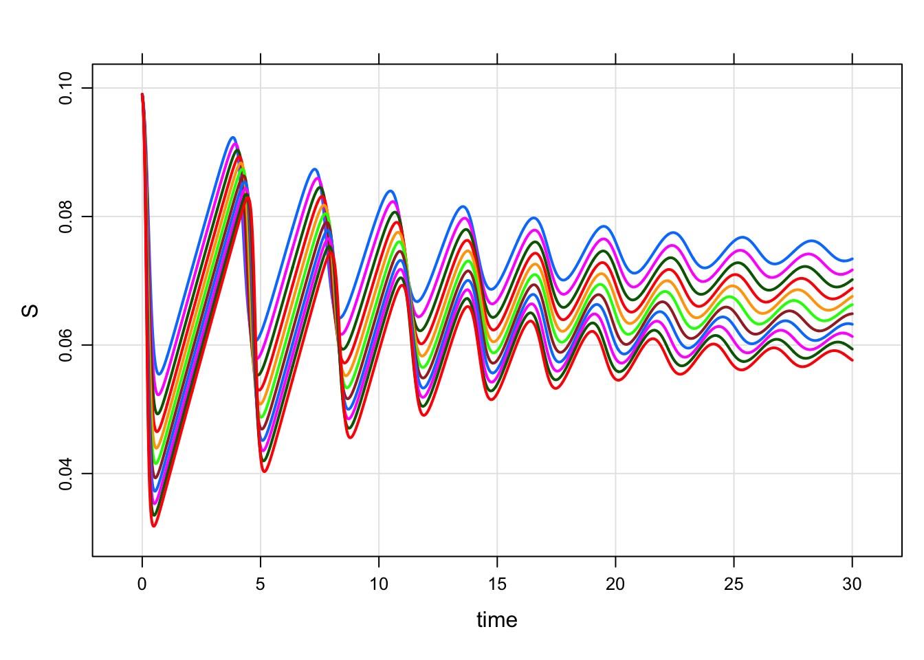
idata <- tibble(Beta = seq(350,450,10))

mod %>% 
  idata_set(idata) %>% 
  mrgsim() %>% 
  plot(S~time)