library(dplyr)
library(mrgsolve)

1 Introduction

This blog post shows some of the new features that came into mrgsolve starting with version 0.10.0 (October 2019) and 0.10.1 (February 2020). The purpose is to illustrate what is possible rather than detailed documentation.

2 Steady-state

This is a big topic, so I put together a separate blog entry to look at new features around steady state.

3 house is now exported

Since the beginning, we have maintained a model inside mrgsolve itself that we call house. It’s a basic PKPD model that we use to test and demo. The interesting thing about this model is that it is compiled when mrgsolve is installed. So the model is always ready to go.

It use to be unexported so you would have to access the model like this:

mod <- mrgsolve:::house()

The ::: means that we go into the mrgsolve namespace to call the function that returns the model object.

Now, house is exported

mod <- house()

4 select_sims

There is a series of dplyr-like functions that allow you to work on the simulation output object (mrgsims) while keeping it a simulation output object. Starting in version 0.10.1, we have a select_sims function which allows you to select certain columns in the simulation object

out <- mrgsim(house(), ev(amt = 100))

out

Model:  housemodel 
Dim:    482 x 7 
Time:   0 to 120 
ID:     1 
    ID time    GUT  CENT  RESP    DV    CP
1:   1 0.00   0.00  0.00 50.00 0.000 0.000
2:   1 0.00 100.00  0.00 50.00 0.000 0.000
3:   1 0.25  74.08 25.75 48.68 1.287 1.287
4:   1 0.50  54.88 44.50 46.18 2.225 2.225
5:   1 0.75  40.66 58.08 43.61 2.904 2.904
6:   1 1.00  30.12 67.83 41.38 3.391 3.391
7:   1 1.25  22.31 74.74 39.58 3.737 3.737
8:   1 1.50  16.53 79.56 38.18 3.978 3.978

out <- select_sims(out, RESP, CP)

out

Model:  housemodel 
Dim:    482 x 4 
Time:   0 to 120 
ID:     1 
    ID time  RESP    CP
1:   1 0.00 50.00 0.000
2:   1 0.00 50.00 0.000
3:   1 0.25 48.68 1.287
4:   1 0.50 46.18 2.225
5:   1 0.75 43.61 2.904
6:   1 1.00 41.38 3.391
7:   1 1.25 39.58 3.737
8:   1 1.50 38.18 3.978

Notice that ID and time are retained. The motivation here is to allow you to request many columns and then pare back so that, for example, plotting is more convenient

plot(out)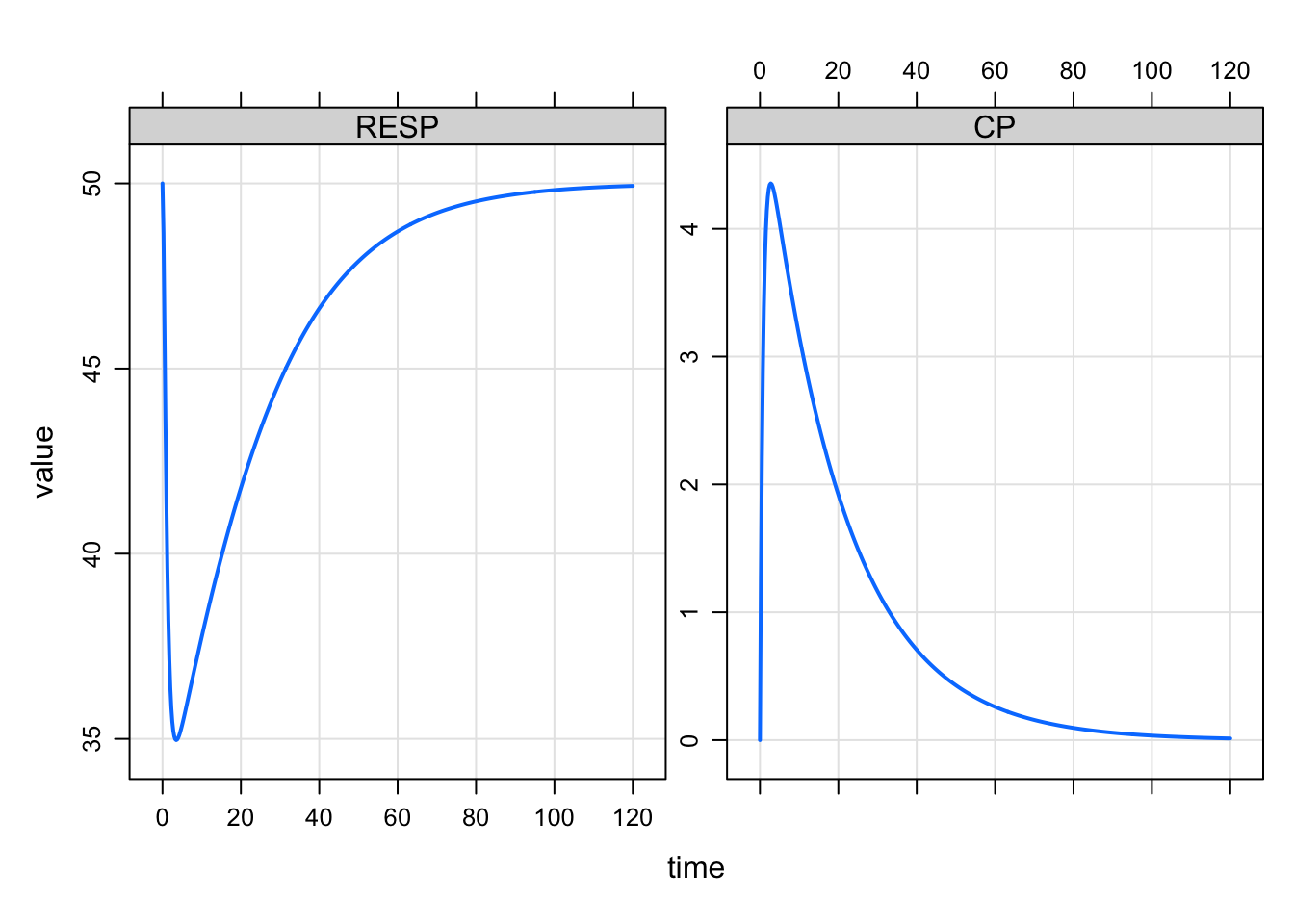

Other functions include

mutate_sims(out, name = "kyle")

Model:  housemodel 
Dim:    482 x 5 
Time:   0 to 120 
ID:     1 
    ID time  RESP    CP name
1:   1 0.00 50.00 0.000 kyle
2:   1 0.00 50.00 0.000 kyle
3:   1 0.25 48.68 1.287 kyle
4:   1 0.50 46.18 2.225 kyle
5:   1 0.75 43.61 2.904 kyle
6:   1 1.00 41.38 3.391 kyle
7:   1 1.25 39.58 3.737 kyle
8:   1 1.50 38.18 3.978 kyle

filter_sims(out, time > 2)

Model:  housemodel 
Dim:    472 x 4 
Time:   2.25 to 120 
ID:     1 
    ID time  RESP    CP
1:   1 2.25 35.84 4.312
2:   1 2.50 35.46 4.345
3:   1 2.75 35.22 4.355
4:   1 3.00 35.07 4.348
5:   1 3.25 34.99 4.329
6:   1 3.50 34.97 4.302
7:   1 3.75 34.98 4.267
8:   1 4.00 35.03 4.229

Notice in all of these operations, the mrgsims object is returned. If you want to mutate or select and get a tibble back, then just call

mutate(out, name = "Kyle")

# A tibble: 482 × 5
      ID  time  RESP    CP name 
   <dbl> <dbl> <dbl> <dbl> <chr>
 1     1  0     50    0    Kyle 
 2     1  0     50    0    Kyle 
 3     1  0.25  48.7  1.29 Kyle 
 4     1  0.5   46.2  2.23 Kyle 
 5     1  0.75  43.6  2.90 Kyle 
 6     1  1     41.4  3.39 Kyle 
 7     1  1.25  39.6  3.74 Kyle 
 8     1  1.5   38.2  3.98 Kyle 
 9     1  1.75  37.1  4.14 Kyle 
10     1  2     36.4  4.25 Kyle 
# ℹ 472 more rows

5 Plot from character vector of column names

The plot method has so far required you to enter a formula to select columns to plot

out <- mrgsim(house(), ev(amt = 100))

plot(out, CP~time)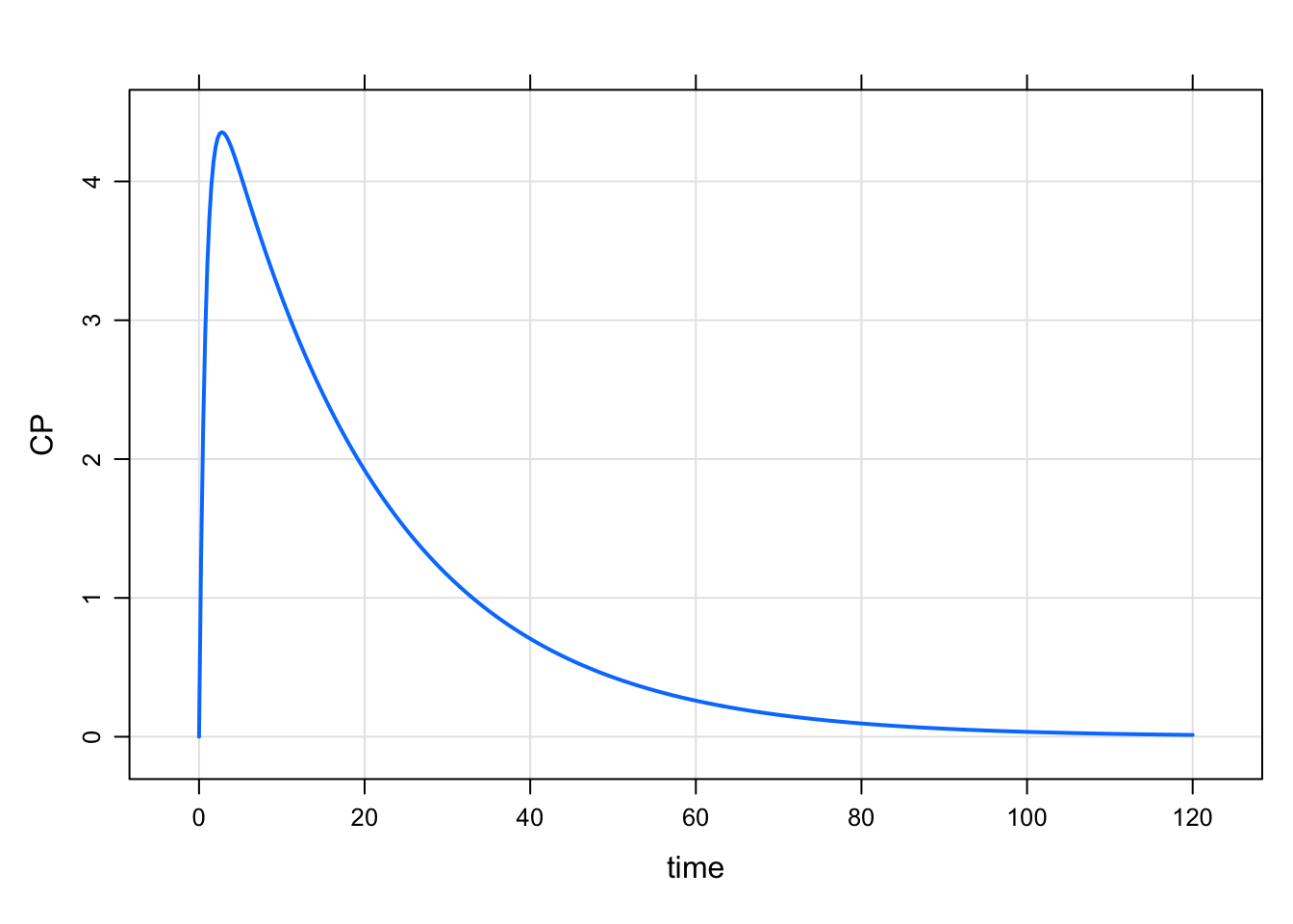

This works well is many circumstances. The new feature here is that you can list the columns to plot as a character vector. Let’s mrgsolve determine what column to put on the x-axis

plot(out, "CP RESP GUT")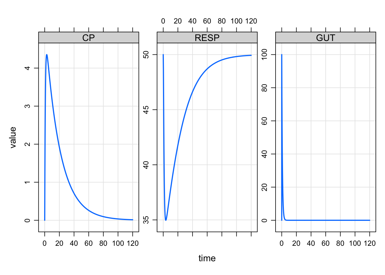

The motivation came from simulations that I was doing where there were a lot of columns in the output and I had many different panel plots I wanted to make. It was helpful to select the columns in a character vector rather than typing out the formula

mod <- modlib("pbpk")

Building pbpk ... done.

out <- mrgsim(mod, ev(amt = 100))

set1 <- "Aad Abo Abr Ahe"
set2 <- "Ave Are Ask Asp Ali Aki"

plot(out, set1)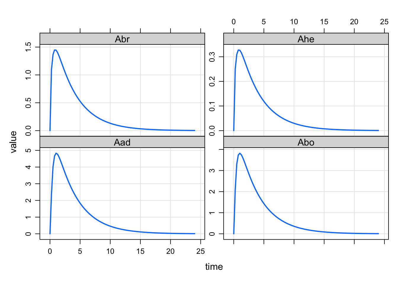

plot(out, set2)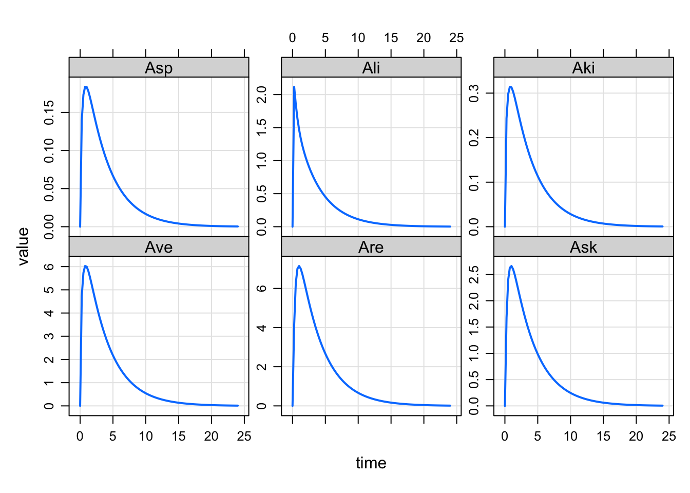

As you expect with mrgsolve, there is no need to specify a real R vector for listing the column names. We’ll split a string on space or comma. For this feature, we’ll also split on newline (helpful when the names are very long or you just want some structure to the layout

set3 <- '
  Aad Abo Abr Ahe
  Ave Are Ask Asp Ali Aki
'

plot(out, set3)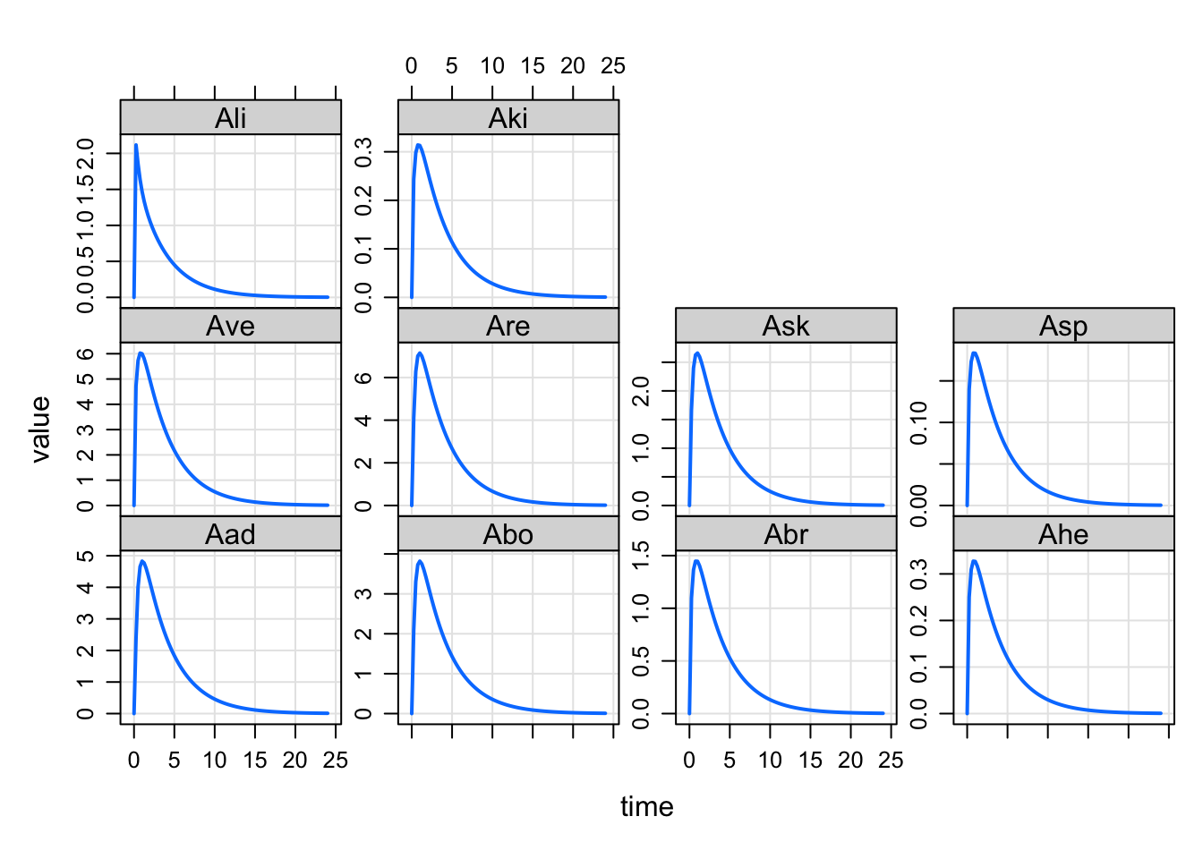

6 outvars

Query the model object for the names of variables that you could ask for in a simulation

outvars(house())

$cmt
[1] "GUT"  "CENT" "RESP"

$capture
[1] "DV" "CP"

Some names are compartments, some are captured.

7 Improvements to event objects

To make an event object

ev(amt = 100)

Events:
  time amt cmt evid
1    0 100   1    1

We can reference names in the object during construction

ev(amt = 100, rate = amt/2)

Events:
  time amt rate cmt evid
1    0 100   50   1    1

I can also access columns in the event object

x <- ev(amt = 100, rate = amt/3)
x$rate

[1] 33.33333

And we have been able to mutate these objects for a while now

x <- ev(amt = 100) 

mutate(x, rate = amt / 5)

Events:
  time amt rate cmt evid
1    0 100   20   1    1

Check out the tinf argument to say how long you want an infusion to last

ev(amt = 100, tinf = 3)

Events:
  time amt     rate cmt evid tinf
1    0 100 33.33333   1    1    3

8 New error message

You might see this

dose <- ev(amt = 100)

try(mrgsim(dose, mod))

Error : the first argument to mrgsim must be a model object

Which just means you passed things in in the wrong order.

9 Steady state infusion

mrgsolve can now run a zero-order infusion to steady state. Set amt to 0, rate to something positive and ss to 1. We change recsort just to show that things start at steady state.

ssinf <- ev(amt = 0, rate = 5, ss = 1)

mrgsim(house(), event = ssinf, recsort=3) %>% plot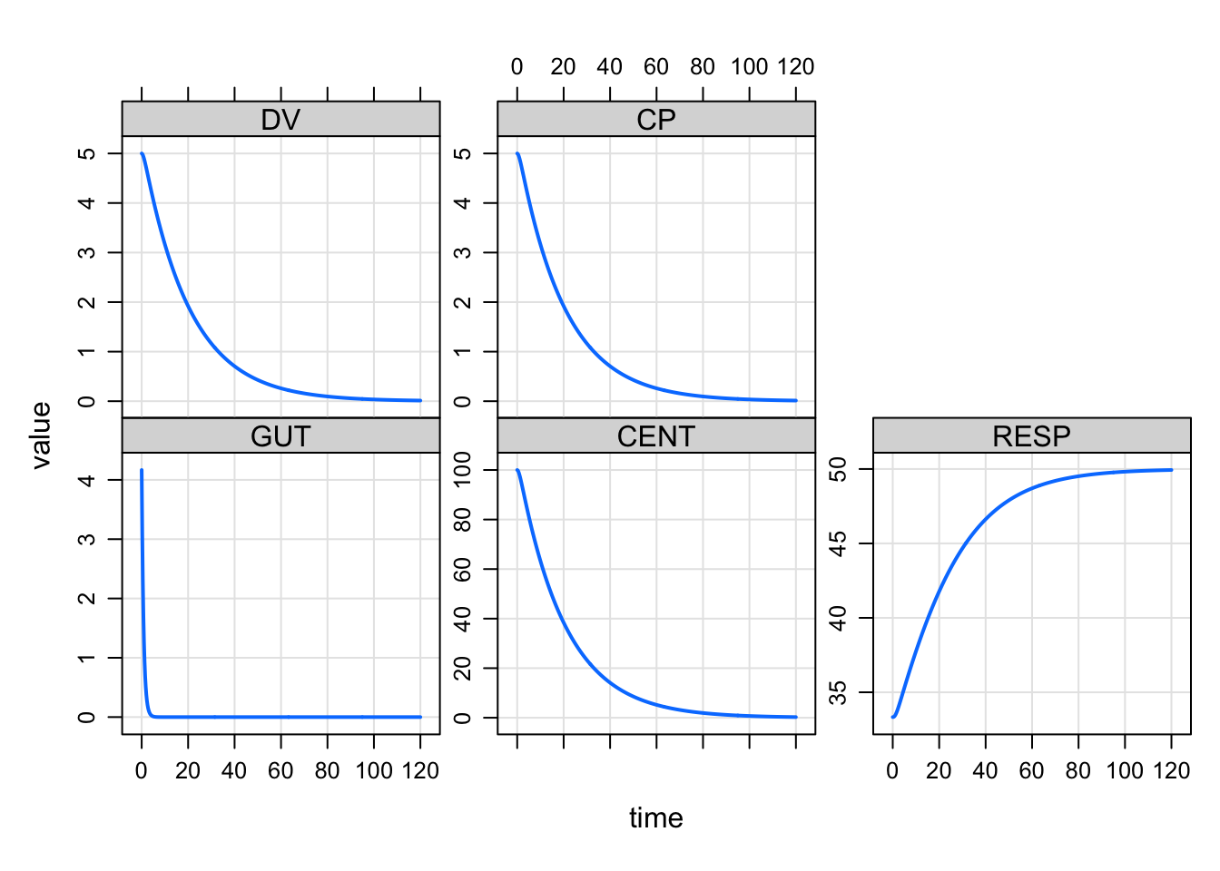

You can also set rate to -1 if you are modeling the rate. But it can’t be set to -2.

10 Access model information

For a while, you could access model parameters with $ operator

mod <- house()

mod$CL

[1] 1

Now you can access initial compartment values

mod$RESP

[1] 50

And other goodies

mod$end

[1] 120

11 Access compartment numbers

Sometimes when writing a model, we would like to know the number of a compartment when we only know the name. There is a plugin to make that doable now

$CMT CENTRAL

$PLUGIN N_CMT

$MAIN

if(CMT==N_CENTRAL) {
  // ......
}