library(msm)
library(mrgsolve)
library(dplyr)
library(minqa)
options(pillar.width = Inf)1 Introduction
This post shows how you can fit a simple multi-state model with mrgsolve. We’ll fit a model to the cav data from the msm package using both msm and mrgsolve and then compare the results.
Some references for the data and analysis include
Sharples, L. D., Jackson, C. H., Parameshwar, J., Wallwork, J. & Large, S. R. Diagnostic accuracy of coronary angiography and risk factors for post-heart-transplant cardiac allograft vasculopathy. Transplantation 76, 679–682 (2003). [Link]
Jackson, C. H. Multi-State Models for Panel Data: The msm Package for R. J. Stat. Softw. 38, 1–28 (2011). [Link]
Multi-state modelling in R: the
msmpackage [Link]
This post updated July 2024 to use mrgsolve 1.5.1 which introduces a replace() function in the evt namespace (see the evtools plugin). The evt::replace() syntax is just like evt::bolus(), but we replace the the amount in the indicated compartment, rather than adding to it. This utilizes EVID = 8, a long-standing feature in mrgsolve, which can be conveniently called from within your model starting with 1.5.1.
The cav data is a “series of approximately yearly angiographic examinations of heart transplant recipients. The state at each time is a grade of cardiac allograft vasculopathy (CAV), a deterioration of the arterial walls.” (Link).
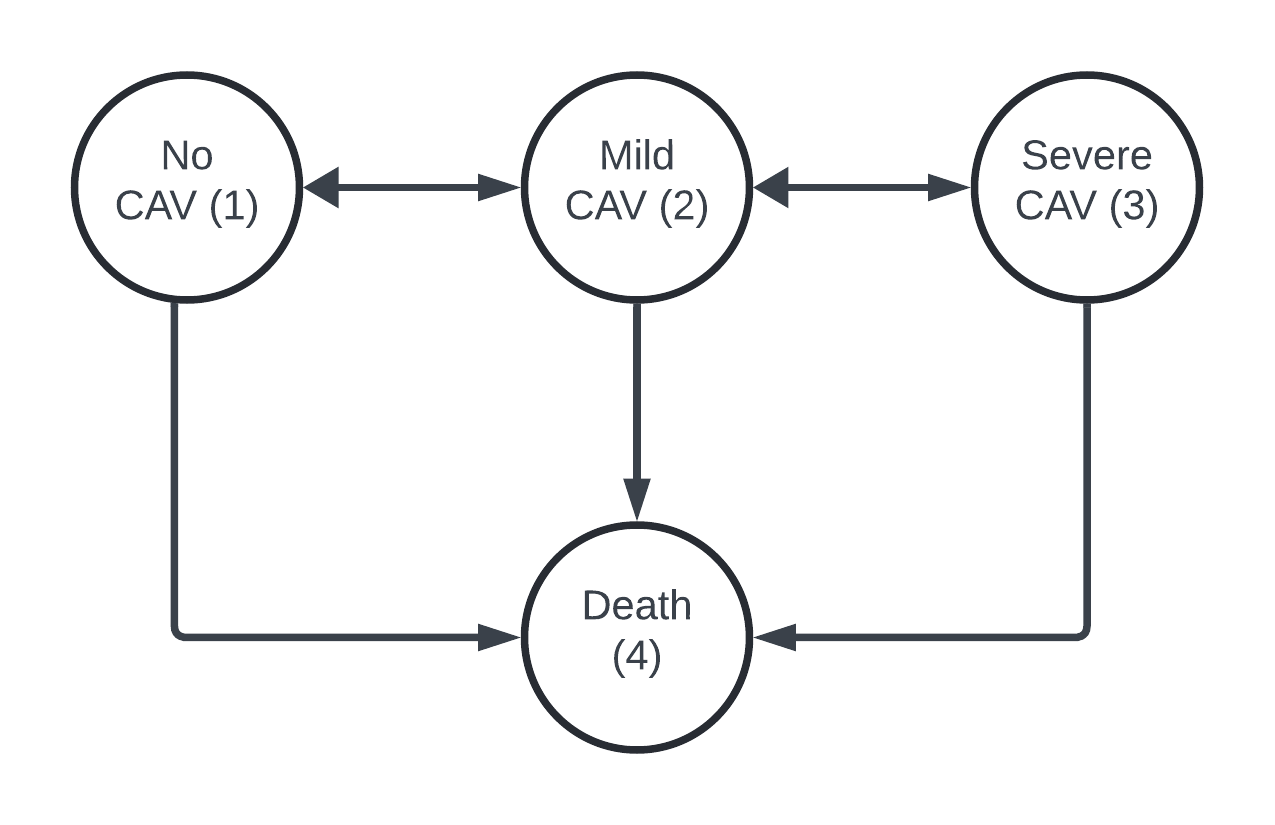
There are four states in the CAV data set
- No CAV
- Mild or moderate CAV
- Severe CAV
- Death
The data set includes 2846 observations across 622 subjects.
2 Fit the model with msm
2.1 Transition matrix
The transitions in the data set look like
statetable.msm(state, PTNUM, data=cav) to
from 1 2 3 4
1 1367 204 44 148
2 46 134 54 48
3 4 13 107 55We’ll follow the analysis presented by the msm package, using this transition matrix
qq <- rbind(
  c(0, 0.25, 0, 0.25),
  c(0.166, 0, 0.166, 0.166),
  c(0, 0.25, 0, 0.25),
  c(0, 0, 0, 0)
)
qq
[,1] [,2] [,3] [,4]
[1,] 0.000 0.25 0.000 0.250
[2,] 0.166 0.00 0.166 0.166
[3,] 0.000 0.25 0.000 0.250
[4,] 0.000 0.00 0.000 0.000This assumes that transitions between State 1 and State 3 must pass through State 2.
2.2 Call to fit the model
Fit the model with deathexact = 4, indicating that 4 (death) is an absorbing state whose time of entry is known exactly, but with unknown transient state just prior to entering.
cav.msm <- msm(
  state ~ years,
  subject = PTNUM,
  data = cav,
  qmatrix = qq,
  deathexact = 4
)

cav.msm
Call:
msm(formula = state ~ years, subject = PTNUM, data = cav, qmatrix = qq,     deathexact = 4)

Maximum likelihood estimates

Transition intensities
                  Baseline
State 1 - State 1 -0.17037 (-0.19027,-0.15255)
State 1 - State 2  0.12787 ( 0.11135, 0.14684)
State 1 - State 4  0.04250 ( 0.03412, 0.05294)
State 2 - State 1  0.22512 ( 0.16755, 0.30247)
State 2 - State 2 -0.60794 (-0.70880,-0.52143)
State 2 - State 3  0.34261 ( 0.27317, 0.42970)
State 2 - State 4  0.04021 ( 0.01129, 0.14324)
State 3 - State 2  0.13062 ( 0.07952, 0.21457)
State 3 - State 3 -0.43710 (-0.55292,-0.34554)
State 3 - State 4  0.30648 ( 0.23822, 0.39429)

-2 * log-likelihood:  3968.798
The msm package provides some visualization of the result
plot(cav.msm)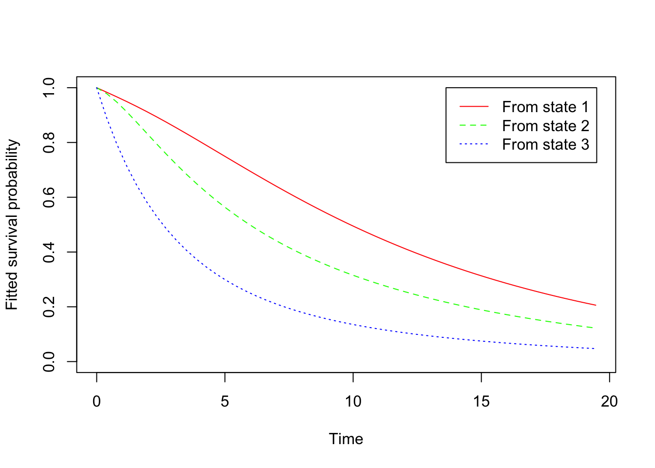
3 Now use mrgsolve
3.1 Data
Modify the data to use with mrgsolve, adding columns for ID and TIME
data <- rename(
  as_tibble(cav),
  ID = PTNUM,
  time = years
)
The data set is really fairly simple
head(data, n = 4)# A tibble: 4 × 10
ID age time dage sex pdiag cumrej state firstobs statemax
<int> <dbl> <dbl> <int> <int> <fct> <int> <int> <int> <dbl>
1 100002 52.5 0 21 0 IHD 0 1 1 1
2 100002 53.5 1.00 21 0 IHD 2 1 0 1
3 100002 54.5 2.00 21 0 IHD 2 2 0 2
4 100002 55.6 3.09 21 0 IHD 2 2 0 2- The
statecolumn marks the state at the examination, ranging from 1 (no CAV) to 3 (severe CAV) as well as State 4 (death). - Every subject starts in
state1 - There are also some covariates that we won’t use in this example
You can also verify that there are no records in the data set to reset or dose into any compartment; we’ll handle all of that from inside the model.
3.2 Model
Set up a model with the four states
msm-cav.mod
$PLUGIN autodec evtools

$CMT @annotated
A1 : 0 : No CAV
A2 : 0 : Mild or moderate CAV
A3 : 0 : Severe CAV
A4 : 0 : Death

$PARAM @annotated
k12 : 0.1 : None to mild or moderate
k21 : 0.1 : Mild or moderate to none
k23 : 0.1 : Mild or moderate to severe
k32 : 0.1 : Severe to mild or moderate
k14 : 0.1 : None to death
k24 : 0.1 : Mild or moderate to death
k34 : 0.1 : Severe to death

$INPUT
state = 1

$PK
A1_0 = 1;

$DES
dxdt_A1 = -A1 * k12 + A2 * k21 - A1 * k14;
dxdt_A2 =  A1 * k12 - A2 * k21 - A2 * k23 + A3 * k32 - A2 * k24;
dxdt_A3 =  A2 * k23 - A3 * k32 - A3 * k34;
dxdt_A4 =  A1 * k14 + A2 * k24 + A3 * k34;

$ERROR
if(EVID != 0) return;

if(state==1) Y = A1;
if(state==2) Y = A2;
if(state==3) Y = A3;
if(state==4) Y = A1 * k14 + A2 * k24 + A3 * k34;

for(int st = 1; st <= 4; ++st) {
  evt::replace(self, 0, st);
}
evt::bolus(self, 1, state);

$CAPTURE Y
The key to this model is the evt::replace() function, which will reset all compartments to 0 when there is an examination and then initialize the appropriate compartment with a 1 based on the value of state in the data set. We do this with a simple for loop in C++. The replace() functionality is available in the evtools plugin starting with mrgsolve 1.5.1. More on evtools in the mrgsolve user guide.
3.3 Call to fit the model
Load the model and set up for estimation
mod <- mread("msm-cav.mod")The initial estimates will be whatever we wrote into the model file
theta <- as.numeric(param(mod))
theta <- theta[grep("^k", names(theta))]
tnames <- names(theta)
This function takes in a set of parameters and returns the -2 log-likelihood returned from the model.
ofv <- function(p, data) {
  p <- lapply(p, exp)
  names(p) <- tnames
  mod <- param(mod, p)
  out <- mrgsim_q(mod, data)
  -2*sum(log(out$Y))
}
Use minqa::newuoa() to fit the model
fit <- newuoa(
  par = log(theta),
  fn = ofv,
  data = data,
  control = list(iprint = 1)
)
start par. = -2.302585 -2.302585 -2.302585 -2.302585 -2.302585 -2.302585 -2.302585 fn = 4208.405
At return
eval: 247 fn: 3968.7979 par: -2.05671 -1.49120 -1.07120 -2.03544 -3.15859 -3.21225 -1.18267This takes 4 to 4.5 seconds on my MacBook M1 Pro.
4 Compare msm and mrgsolve results
The final objective function values for the msm and mrgsolve fits are similar
fit$fval[1] 3968.79787942cav.msm$minus2loglik[1] 3968.79789305Compare estimated transition intensities (there might be a naming issue on the cav.msm estimates, but I think the values match up).
est <- exp(fit$par)

names(est) <- tnames

est %>% sort()
k24 k14 k12 k32 k21 k34 k23
0.04026573 0.04248539 0.12787425 0.13062362 0.22510161 0.30645974 0.34259570 exp(cav.msm$estimates) %>% sort() qbase qbase qbase qbase qbase qbase qbase
0.04021023 0.04250042 0.12787033 0.13062235 0.22511913 0.30647512 0.34261129