1 Introduction

This post introduces a new formal code block for writing models where there are no compartments. The block is named after the analogous NONMEM block called $PRED. This functionality has always been possible with mrgsolve, but only now is there a code block dedicated to these models. Also, a relaxed set of data set constraints have been put in place when these types of models are invoked.

2 Example model

As a most-basic model, we look at the pred1 model in modlib()

library(mrgsolve)
options(mrgsolve.soloc="build")
mod <- mread_cache("pred1", modlib())

The model code is

$PROB
An example model expressed in closed form
$PARAM B = -1, beta0 = 100, beta1 = 0.1
$OMEGA 2 0.3
$PRED
double beta0i = beta0 + ETA(1);
double beta1i = beta1*exp(ETA(2));
capture Y = beta0i + beta1i*B;

This is a random-intercept, random slope linear model. Like other models in mrgsolve, you can write parameters ($PARAM), and random effects ($OMEGA). But the model is actually written in $PRED.

When mrgsolve finds $PRED, it will generate an error if it also finds $MAIN, $TABLE, or $ODE. However, the code that gets entered into $PRED would function exactly as if you put it in $TABLE.

In the example model, the response is a function of the parameter B, so we’ll generate an input data set with some values of B

library(dplyr)
data <- tibble(ID = 1, B = exp(rnorm(100, 0,2)))

head(data)

# A tibble: 6 × 2
     ID       B
  <dbl>   <dbl>
1     1   3.76 
2     1 196.   
3     1   2.90 
4     1   0.168
5     1   0.278
6     1   0.773

out <- mrgsim_d(mod,data,carry.out="B")

plot(out, Y~B)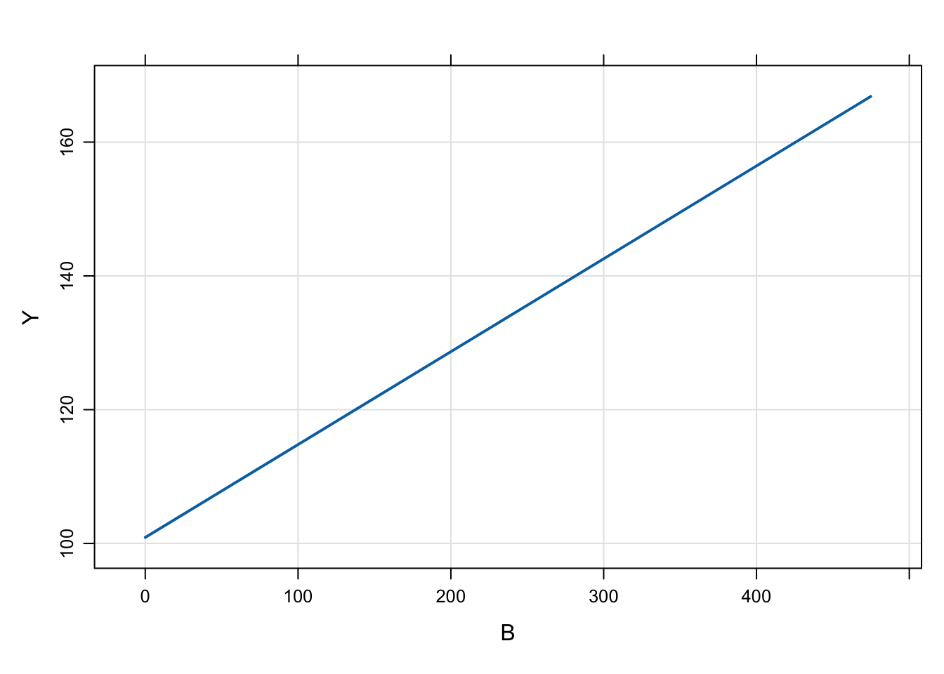

Like other models, we can simulate from a population

library(purrr)
set.seed(223)
df <- map_df(1:30, function(i) tibble(ID = i, B = seq(0,30,1)))

head(df)

# A tibble: 6 × 2
     ID     B
  <int> <dbl>
1     1     0
2     1     1
3     1     2
4     1     3
5     1     4
6     1     5

mod %>% 
  data_set(df) %>% 
  mrgsim(carry.out="B") %>%
  plot(Y ~ B)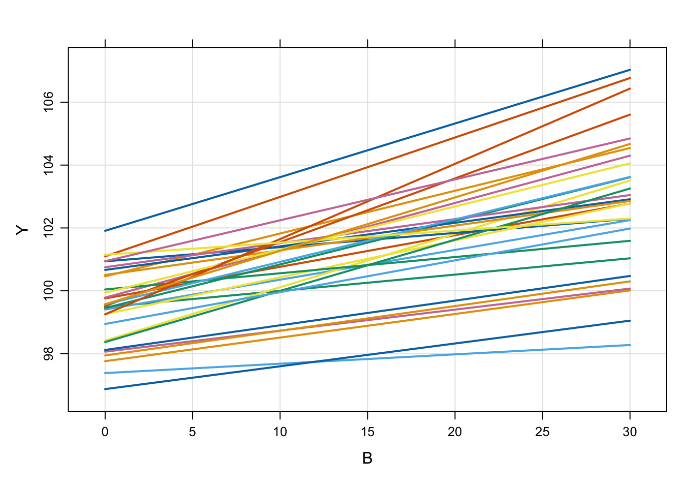

3 PK/PD Model

Here is an implementation of a PK/PD model using $PRED

In this model

Calculate CL as a function of WT and a random effect
Derive AUC from CL and DOSE
The response (Y) is a calculated from AUC and the Emax model parameters

code <- '
$PARAM TVCL = 1, WT = 70, AUC50 = 20, DOSE = 100, E0 = 35, EMAX = 2.4

$OMEGA 1

$SIGMA 100

$PRED
double CL = TVCL*pow(WT/70,0.75)*exp(ETA(1));
capture AUC = DOSE/CL;
capture Y = E0*(1+EMAX*AUC/(AUC50+AUC))+EPS(1);
'

mod <- mcode_cache("pkpd", code)

Loading model from cache.

To simulate, look at 50 subjects at each of 5 doses

data <- 
  expand.idata(DOSE = c(30,50,80,110,200),ID = 1:50) %>% 
  mutate(WT = exp(rnorm(n(),log(80),1)))

head(data)

  ID DOSE        WT
1  1   30  59.13254
2  2   50 317.32739
3  3   80 242.15746
4  4  110 170.78136
5  5  200 248.18054
6  6   30  51.22012

out <- mrgsim_d(mod,data,carry.out="WT,DOSE") %>% as.data.frame

head(out)

  ID time        WT DOSE       AUC         Y
1  1    0  59.13254   30 231.90852 110.61330
2  2    0 317.32739   50  36.76051  85.27834
3  3    0 242.15746   80  36.54808  98.90407
4  4    0 170.78136  110  23.68354  80.29131
5  5    0 248.18054  200 331.10229 108.81926
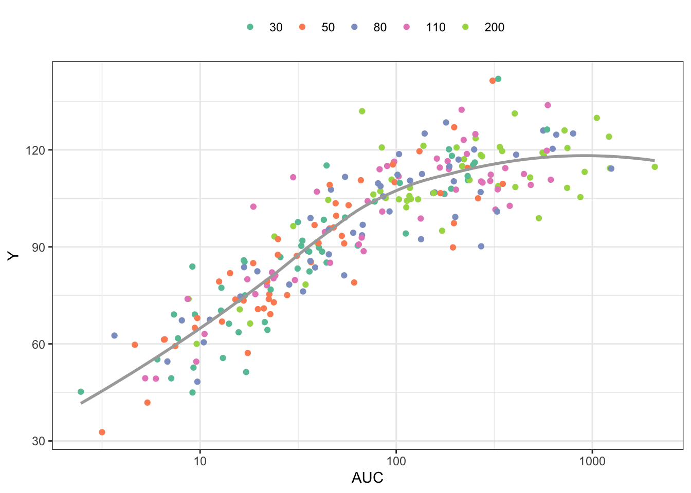
6  6    0  51.22012   30 251.58373 116.09649

Plot the response (Y) versus AUC, colored by dose

library(ggplot2)

ggplot(out, aes(AUC,Y,col =factor(DOSE))) + 
  geom_point() + 
  scale_x_continuous(trans = "log", breaks = 10^seq(-4,4)) + 
  geom_smooth(aes(AUC,Y),se = FALSE,col="darkgrey") + theme_bw() + 
  scale_color_brewer(palette = "Set2", name = "") + 
  theme(legend.position = "top")

`geom_smooth()` using method = 'loess' and formula = 'y ~ x'