Models without compartments ($PRED)

This vignette introduces a new formal code block for writing models where there are no compartments. The block is named after the analogous NONMEM block called $PRED. This functionality has always been possible with mrgsolve, but only now is there a code block dedicated to these models. Also, a relaxed set of data set constraints have been put in place when these types of models are invoked.

Status

The functionality in this vignette can only be access from the GitHub version. We will update this vignette once these features are rolled into a release on CRAN.

Example model

As a most-basic model, we look at the pred1 model in modlib()

library(mrgsolve)
mod <- modlib("pred1")

The model code is

$PROB
An example model expressed in closed form
$PARAM B = -1, beta0 = 100, beta1 = 0.1
$OMEGA 2 0.3
$PRED
double beta0i = beta0 + ETA(1);
double beta1i = beta1*exp(ETA(2));
capture Y = beta0i + beta1i*B;

This is a random-intercept, random slope linear model. Like other models in mrgsolve, you can write parameters ($PARAM), and random effects ($OMEGA). But the model is actually written in $PRED.

When mrgsolve finds $PRED, it will generate an error if it also finds $MAIN, $TABLE, or $ODE. However, the code that gets entered into $PRED would function exactly as if you put it in $TABLE.

In the example model, the response is a function of the parameter B, so we’ll generate an input data set with some values of B

library(dplyr)
data <- data_frame(ID = 1, B = exp(rnorm(100, 0,2)))

Warning: `data_frame()` was deprecated in tibble 1.1.0.
ℹ Please use `tibble()` instead.

head(data)

# A tibble: 6 × 2
     ID      B
  <dbl>  <dbl>
1     1  2.83 
2     1  2.36 
3     1  0.331
4     1  0.466
5     1  8.34 
6     1 39.6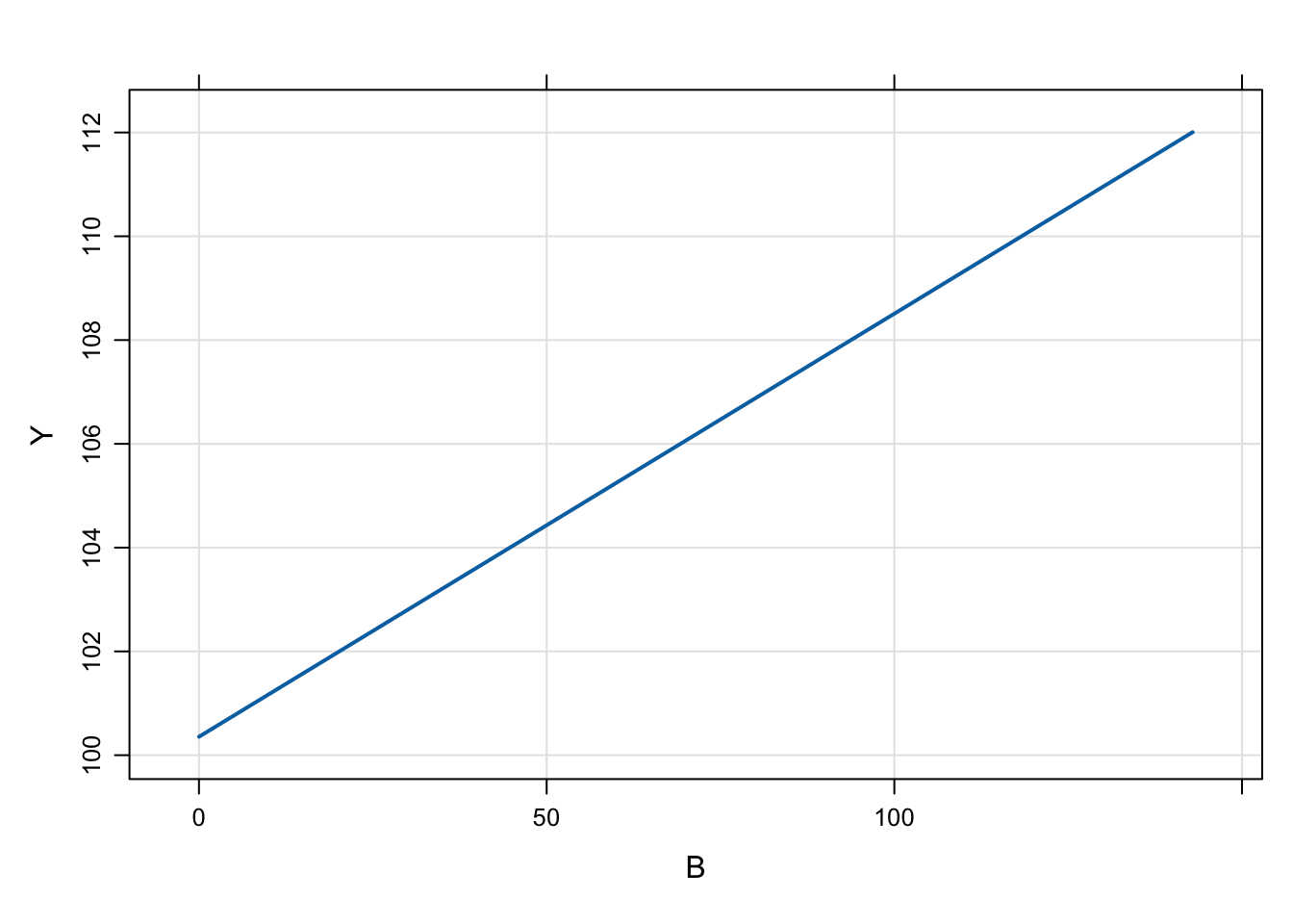

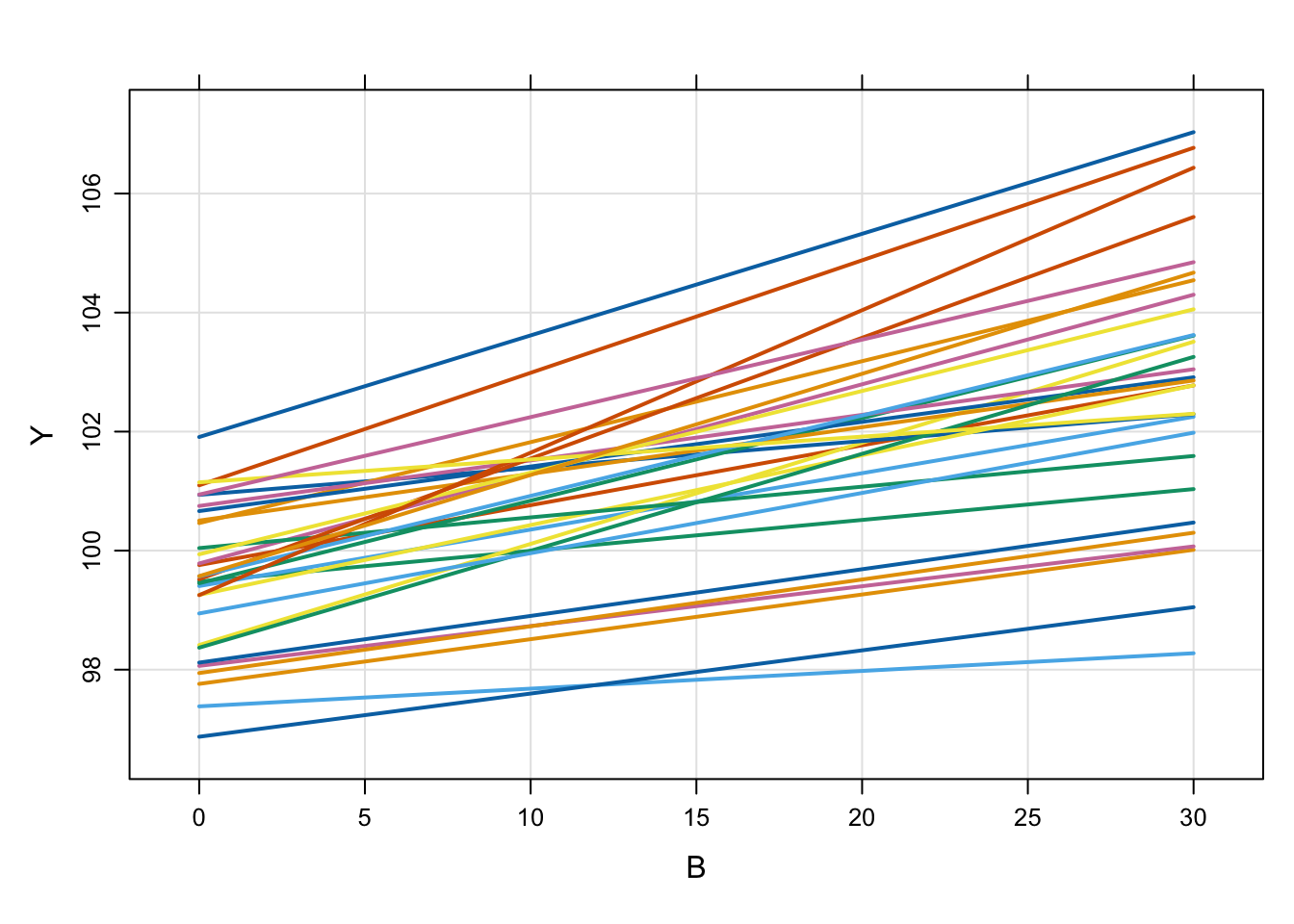
out <- mrgsim_d(mod,data,carry.out="B")

plot(out, Y~B)

Like other models, we can simulate from a population

library(purrr)
set.seed(223)
df <- map_df(1:30, function(i) data_frame(ID = i, B = seq(0,30,1)))

head(df)

# A tibble: 6 × 2
     ID     B
  <int> <dbl>
1     1     0
2     1     1
3     1     2
4     1     3
5     1     4
6     1     5

mod %>% 
  data_set(df) %>% 
  mrgsim(carry.out="B") %>%
  plot(Y ~ B)

PK/PD Model

Here is an implementation of a PK/PD model using $PRED

In this model

Calculate CL as a function of WT and a random effect
Derive AUC from CL and DOSE
The response (Y) is a calculated from AUC and the Emax model parameters

code <- '
$PARAM TVCL = 1, WT = 70, AUC50 = 20, DOSE = 100, E0 = 35, EMAX = 2.4

$OMEGA 1

$SIGMA 100

$PRED
double CL = TVCL*pow(WT/70,0.75)*exp(ETA(1));
capture AUC = DOSE/CL;
capture Y = E0*(1+EMAX*AUC/(AUC50+AUC))+EPS(1);
'

mod <- mcode_cache("pkpd", code)

Building pkpd ... done.

To simulate, look at 50 subjects at each of 5 doses

data <- 
  expand.idata(DOSE = c(30,50,80,110,200),ID = 1:50) %>% 
  mutate(WT = exp(rnorm(n(),log(80),1)))

head(data)

  ID DOSE        WT
1  1   30  59.13254
2  2   50 317.32739
3  3   80 242.15746
4  4  110 170.78136
5  5  200 248.18054
6  6   30  51.22012

out <- mrgsim_d(mod,data,carry.out="WT,DOSE") %>% as.data.frame()

head(out)

  ID time        WT DOSE       AUC         Y
1  1    0  59.13254   30 231.90852 110.61330
2  2    0 317.32739   50  36.76051  85.27834
3  3    0 242.15746   80  36.54808  98.90407
4  4    0 170.78136  110  23.68354  80.29131
5  5    0 248.18054  200 331.10229 108.81926
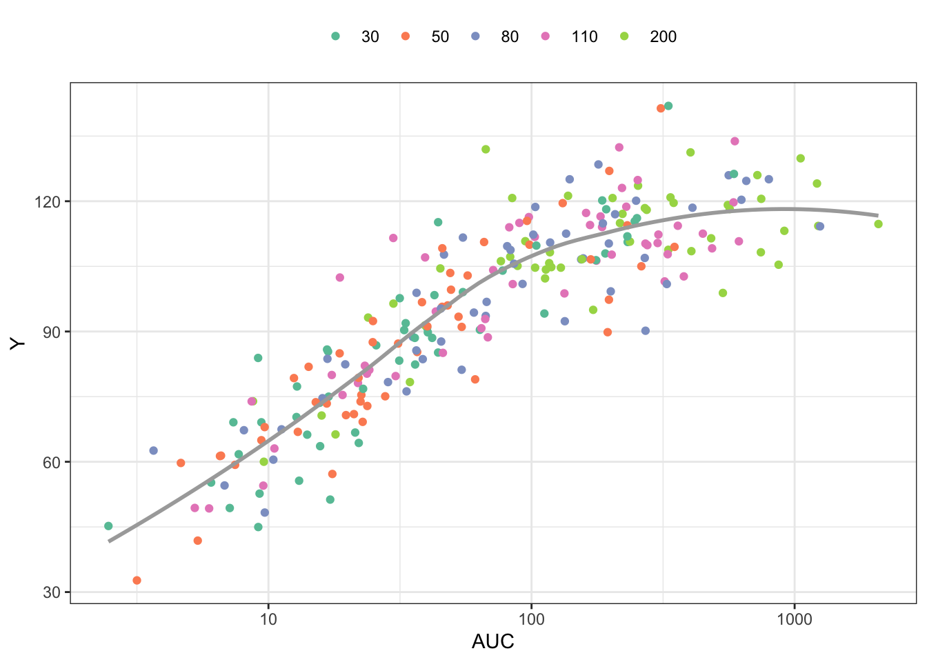
6  6    0  51.22012   30 251.58373 116.09649

Plot the response (Y) versus AUC, colored by dose

library(ggplot2)

ggplot(out, aes(AUC,Y,col =factor(DOSE))) + 
  geom_point() + 
  scale_x_continuous(trans = "log", breaks = 10^seq(-4,4)) + 
  geom_smooth(aes(AUC,Y),se = FALSE,col="darkgrey") + theme_bw() + 
  scale_color_brewer(palette = "Set2", name = "") + 
  theme(legend.position = "top")

`geom_smooth()` using method = 'loess' and formula = 'y ~ x'