Quick Start

This vignette shows the user how to do their first simulation with mrgsolve.

Load a model

After loading the package

library(mrgsolve)

we’ll use the mread() function to read, parse, compile and load a model out of the internal model library. Try calling the modlib function (modlib()) and see that the path to the installed package is returned, pointing to a directory of pre-coded models. These models are good to try when learning mrgsolve.

For this first example, we’re using a one compartment model (called pk1 in the model library)

mod <- modlib("pk1")

Once we create the model object (mod) we can extract certain information about the model. For example, get an overview

mod

. 
. 
. -----------------  source: pk1.cpp  -----------------
. 
.   project: /Users/kyleb/Lib...gsolve/models
.   shared object: pk1-so-f1064908fa6d 
. 
.   time:          start: 0 end: 24 delta: 1
.                  add: <none>
. 
.   compartments:  EV CENT [2]
.   parameters:    CL V KA [3]
.   captures:      CP [1]
.   omega:         0x0 
.   sigma:         0x0 
. 
.   solver:        atol: 1e-08 rtol: 1e-08 maxsteps: 20k
. ------------------------------------------------------

Or look at model parameters and their values

param(mod)

. 
.  Model parameters (N=3):
.  name value . name value
.  CL   1     | V    20   
.  KA   1     | .    .

We’ll see in the section below how to run a simulation from this model. But first, let’s create a dosing intervention to use with this model.

Create an intervention

The simplest way to create an intervention is to use an event object. This is just a simple expression of one or more model interventions (most frequently doses)

evnt <- ev(amt = 100, ii = 24, addl = 9)

evnt

. Events:
.   time amt ii addl cmt evid
. 1    0 100 24    9   1    1

We’ll see in other vignettes how to create more-complicated events as well as how to create larger data sets with many individuals in them.

For now, the event object is just an intervention that we can combine with a model.

Simulate

To simulate, use the mrgsim() function.

out <- mod %>% ev(evnt) %>% mrgsim(end = 480, delta = 0.1)

We use a pipe sequence here (%>%) to pass the model object (mod) into the event function (ev()) where we attach the dosing intervention, and that result gets passed into the simulation function. The result of the simulation function is essentially a data frame of simulated values

out

. Model:  pk1 
. Dim:    4802 x 5 
. Time:   0 to 480 
. ID:     1 
.     ID time     EV   CENT     CP
. 1:   1  0.0   0.00  0.000 0.0000
. 2:   1  0.0 100.00  0.000 0.0000
. 3:   1  0.1  90.48  9.492 0.4746
. 4:   1  0.2  81.87 18.034 0.9017
. 5:   1  0.3  74.08 25.715 1.2858
. 6:   1  0.4  67.03 32.619 1.6309
. 7:   1  0.5  60.65 38.819 1.9409
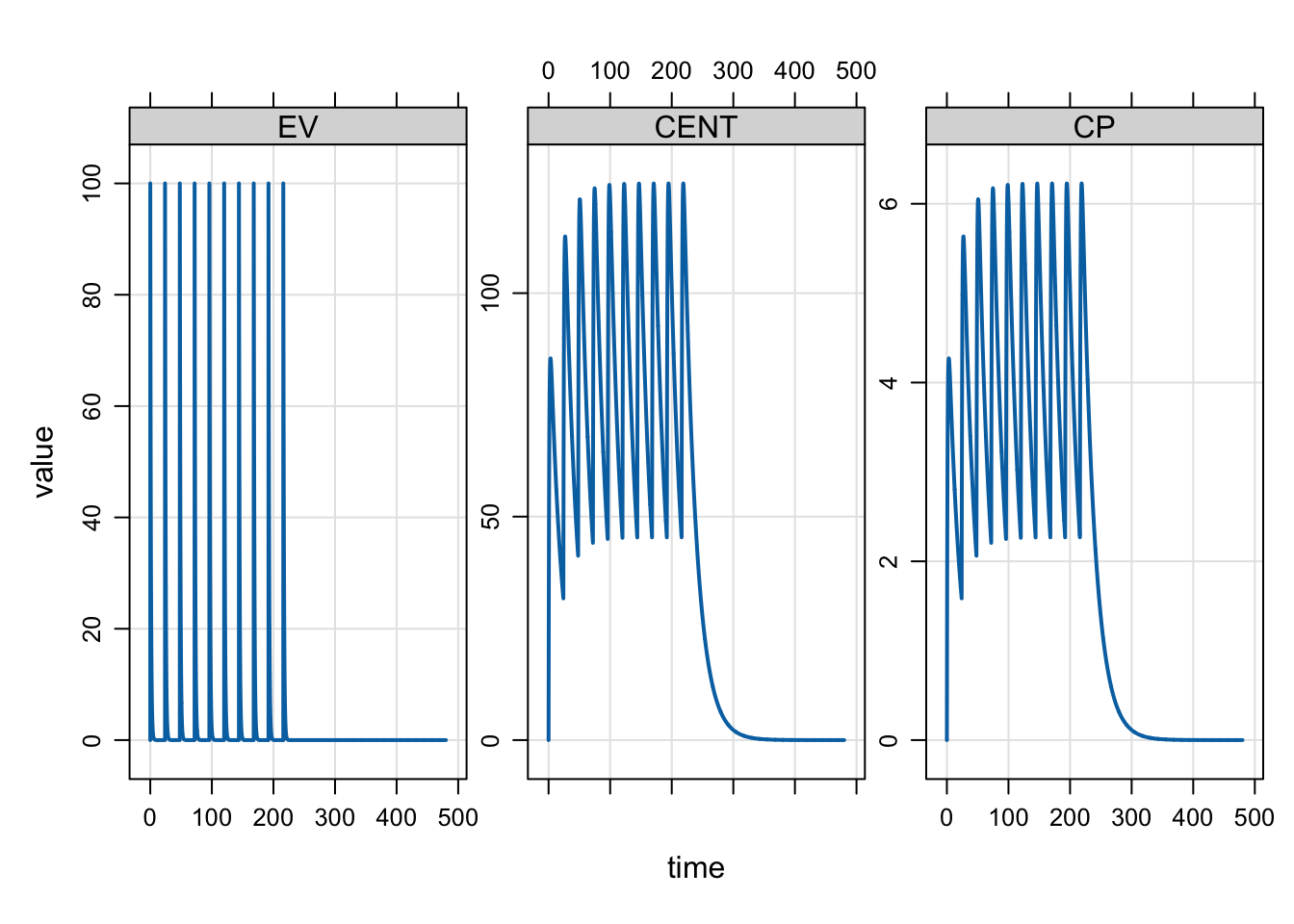
. 8:   1  0.6  54.88 44.383 2.2191

Plot

mrgsolve comes with several different functions for processing output. One simple function is a plot method that will generate a plot of what was just simulated

plot(out)