This is a shortened version of map_bayes.html, showing only the estimation step.

library(ggplot2)
library(mrgsolve)
library(nloptr)
library(dplyr)
library(magrittr)
options(mrgsolve.soloc="build")

1 The model

We code up a one-compartment model, with fixed TVCL and TVV. We have ETA1 and ETA2 as parameters in the model so that we can update them as the optimizer proceeds. Our goal is to find the values of ETA that are most consistent with the data.

code <- '
$SET request=""

$PARAM ETA1 = 0, ETA2 = 0

$CMT CENT

$PKMODEL ncmt=1

$MAIN
double TVCL = 1.5;
double TVVC = 23.4;
double CL = TVCL*exp(ETA1);
double V =  TVVC*exp(ETA2);

$TABLE 
capture DV = (CENT/V);
'

mod <- mcode_cache("map", code)

We also have the OMEGA and SIGMA matrices from the population model estimation step.

omega <- cmat(0.23,-0.78, 0.62)
omega.inv <- solve(omega)
sigma <- matrix(0.0032)

Read in the data set. Notice that DV has value NA for dosing records. When calculating the joint likelihood of all the data, we will remove the missing values (dosing records don’t have observations that contribute to the likelihood value).

data <- readRDS("map_bayes_data.RDS")

head(data)

# A tibble: 4 × 6
     ID  time  evid   amt   cmt    DV
  <dbl> <dbl> <dbl> <dbl> <dbl> <dbl>
1     1   0       1   750     1 NA   
2     1   0.5     0     0     0 42.7 
3     1  12       0     0     0  6.93
4     1  24       0     0     0  1.37

2 Optimize

This function takes in a set of proposed \(\eta\)s along with the observed data vector, the data set and a model object and returns the value of the EBE objective function

When we do the estimation, the fixed effects and random effect variances are fixed.
The estimates are the \(\eta\) for clearance and volume

Arguments:

eta the current values from the optimizer
ycol the observed data column name
d the data set
m the model object
dvcol the predicted data column name
pred if TRUE, just return predicted values

2.1 What is this function doing?

get the matrix for residual error
Make sure eta is a list
Make sure eta is properly named (i.e. ETA1 and ETA2)
Copy eta into a matrix that is one row
Update the model object (m) with the current values of ETA1 and ETA2
Simulate from data set d and save output to out object
If we are just requesting predictions (if(pred)) return the simulated data
The final lines calculate the EBE objective function; see this paper for reference
Notice that the function returns a single value (a number); the optimizer will minimize this value

mapbayes <- function(eta,d,ycol,m,dvcol=ycol,pred=FALSE) {
    
  sig2 <- as.numeric(sigma)
  eta <- as.list(eta)
  names(eta) <- names(init)
  eta_m <- eta %>% unlist %>% matrix(nrow=1)
  m <-  param(m,eta)
  out <- mrgsim(m,data=d,output="df")
  if(pred) return(out)
  # http://www.ncbi.nlm.nih.gov/pmc/articles/PMC3339294/
  sig2j <- out[[dvcol]]^2*sig2
  sqwres <- log(sig2j) + (1/sig2j)*(d[[ycol]] - out[[dvcol]])^2
  nOn <- diag(eta_m %*% omega.inv %*% t(eta_m))
  return(sum(sqwres,na.rm=TRUE) + nOn)
}

2.2 Initial estimate

Note again that we are optimizing the etas here

init <- c(ETA1=-0.3, ETA2=0.2)

Fit the data

newuoa is from the nloptr package
Other optimizers (via optim) could probably also be used

Arguments to newuoa

First: the initial estimates
Second: the function to optimize
The other argument are passed to mapbayes

fit <- nloptr::newuoa(init,mapbayes,ycol="DV",m=mod,d=data)

Here are the final estimates ::: {.cell}

fit$par

[1]  0.4995400 -0.3274858

:::

3 Look at the result

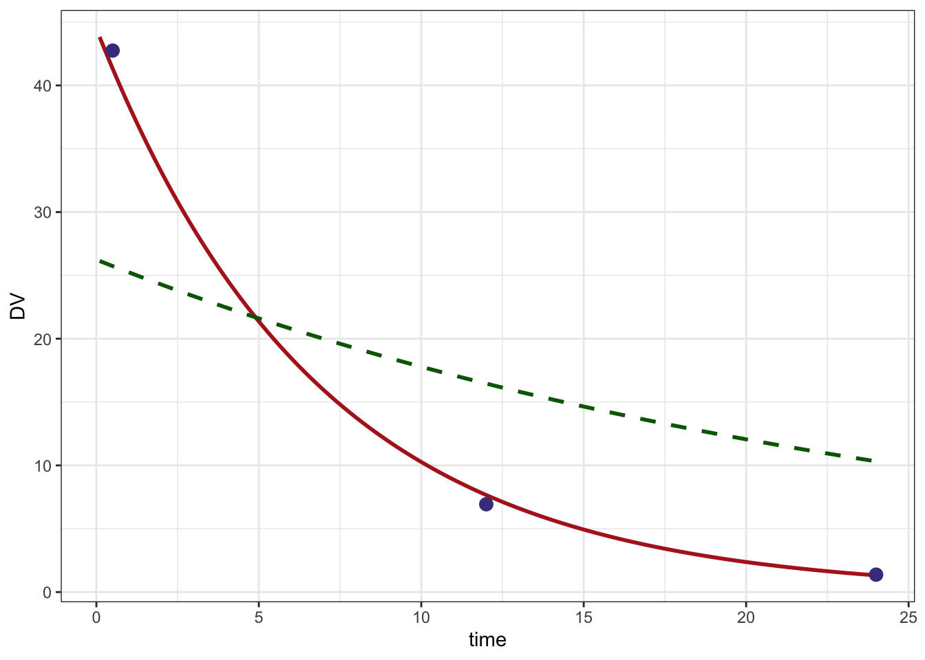
A data set and model to get predictions; this will give us a smooth prediction line

pdata <- data %>% filter(evid==1)
pmod <- mod %>% update(end=24, delta=0.1)

Predicted line based on final estimates ::: {.cell}

pred <- mapbayes(fit$par,ycol="DV",pdata,pmod,pred=TRUE) %>% filter(time > 0)
head(pred)

  ID time       DV
1  1  0.1 43.82331
2  1  0.2 43.18567
3  1  0.3 42.55731
4  1  0.4 41.93809
5  1  0.5 41.32789
6  1  0.6 40.72656

:::

Predicted line based on initial estimates ::: {.cell}

initial <- mapbayes(init,ycol="DV",pdata,pmod,,pred=TRUE) %>% filter(time > 0)
head(initial)

  ID time       DV
1  1  0.1 26.13954
2  1  0.2 26.03811
3  1  0.3 25.93707
4  1  0.4 25.83642
5  1  0.5 25.73616
6  1  0.6 25.63629

:::

Plot ::: {.cell}

ggplot() + 
  geom_line(data=pred, aes(time,DV),col="firebrick", lwd=1) + 
  geom_line(data=initial,aes(time,DV), lty=2, col="darkgreen", lwd=1) + 
  geom_point(data=data %>% filter(evid==0), aes(time,DV), col="darkslateblue",size=3) + 
  theme_bw()

:::