Rmarkdown model specification
1 Introduction
I was an Emacs user for a long time and thought I’d never give it up. But like a lot of other people, Rstudio grew on me and I use it for all my R, C++ and Rcpp work. It just works well.
2 The problem
When I write mrgsolve models, I typically save the code to a file
with .cpp extension (e.g. pkmodel.cpp) so that
I get nice syntax highlighting that Rstudio provides. One thing that
bugs me about this setup is that Rstudio naturally thinks
all the code in pkmodel.cpp is C++ code.
But for mrgsolve models, only part of the code is C++. Other parts are R
or just other syntax that we made up. This means the auto-formatting
that Rstudio does doesn’t always work that great.
3 Some solutions
There are a couple of ways to make this less-irritating. First, you can use brackets for code blocks like this
[ PARAM] CL = 1, V = 20rather than this
$PARAM CL = 1, V = 20I think this helps a bit. You could also save your model to
pkmodel.txt rather than pkmodel.cpp. You will
lose all of the C++ conveniences but Rstudio won’t try to auto-format
your code. This might not be a great solution either.
4 Rmarkdown model specification
Another way to deal with this is to write your model in Rmarkdown
format. This is new in version 0.9.1 and will probably need
some tweaking. But I’m generally happy with the way it’s working so
far.
The models run the same regardless of how you code them. But in the Rmarkdown input format, writing the code might be a little more natural. Also, consistent the the Rmarkdown / literate programming philosophy, you can document your model right as you code the model, but with structured markdown input.
For example you can now load this model
library(mrgsolve)
options(mrgsolve.soloc = "build")

mod <- mread_cache("popex.Rmd", modlib())
This is just a pop-PK model. You can take a closer look at the code here.
mod %>% ev(amt = 100) %>% mrgsim(nid = 30, end = 72) %>% plot()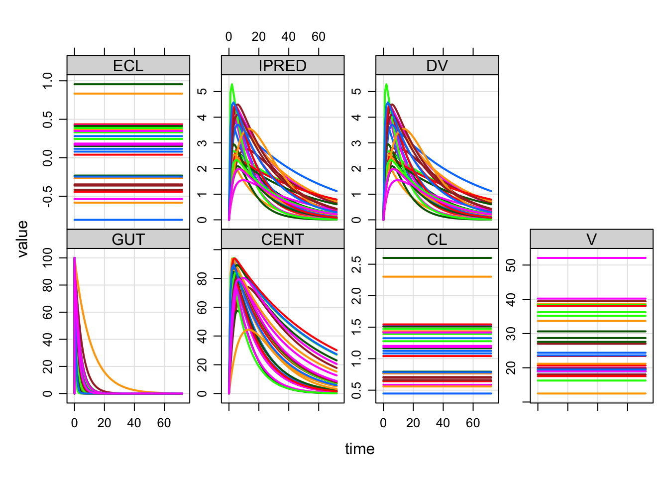
But it’s written in Rmd format
cat(mod@code, sep = "\n"). ---
. title: "Test Rmd model spec"
. output: mrgsolve:::document
. ---
.
. ```{R setup, echo=FALSE}
. knitr::opts_chunk$set(eval=FALSE)
. ```
.
. # Parameters
. ```{param}
. TVKA = 0.5, TVCL = 1, TVV = 24, WT=70
. ```
.
. # OMEGA
. ```{omega}
. @labels ECL EV EKA
. 0.3 0.1 0.5
. ```
.
. # SIGMA
. ```{sigma}
. 0
. ```
.
. # Main block
. ```{main}
. double CL = exp(log(TVCL) + 0.75*log(WT/70) + ECL);
. double V = exp(log(TVV) + log(WT/70) + EV );
. double KA = exp(log(TVKA) + EKA);
. ```
.
. # Model
. ```{pkmodel}
. cmt = "GUT CENT", depot = TRUE
. ```
.
. # Table
. ```{table}
. capture IPRED = CENT/V;
. capture DV = IPRED*exp(EPS(1));
. ```
.
. # Outputs
. ```{capture}
. CL V ECL
. ```At the top of the document, there is regular yaml front matter, with
a title (and optionally date, author etc). I have also included
output which is set to mrgsolve:::document.
The ::: indicates that document is not
exported from the mrgsolve namespace. But using this output lets you
knit this document in Rstudio (with the knit button) and you will get
some html output. This just renders the code into a nice format (with
all the comments and section headers you include in regular old
Rmarkdown format). The mrgsolve:::document output type
defines all sorts of engines like param and
cmt and main and ode etc. These
are block names like you would write in the original input specification
($PARAM and $CMT etc). So only code in
backticks with an engine will be handled as proper model code, the rest
is discarded. There are absolutely no differences in how the code itself
is handled with either the Rmd input format or the traditional input
format. The only difference is the code used to mark the end of one
block and the start of another block.
If you want to write (and evaluate) some R code, use the
R engine.
The only way to properly process a file written like this is if it
has the extension .Rmd or .rmd. So only use
those extensions if you have written your model with the Rmarkdown block
delimiters.
mrgsolve: mrgsolve.github.io | metrum research group: metrumrg.com