Generating input data sets for mrgsolve
library(mrgsolve)
library(dplyr)
1 Input data sets
An important mechanism for creating robust, complex simulations is
the input data set. Input data sets specify the population of
individuals to simulate, including the number of individuals, each
individual’s dosing interventions, each individual’s covariate values
etc. The input data set is just a plain old R
data.frame, but with some expectations about which columns
are present and expectations for how to handle columns for certain
names. For example, every input data set has to have an ID,
time, and cmt column. Note that either lower
case names (like time and cmt) are acceptable
as are upper case names (like TIME and CMT).
But users are not to mix upper and lower case names (like
time and CMT) for certain column names related
to dosing events. The help topic ?data_set discusses more
about what the expectations are for input data sets.
2 Functions to generate input data sets
mrgsolve provides several functions and workflows to help
you put together the right input data set for your simulation. The main
point of this blog post is to review some of these functions to help you
better organize your mrgsolve simulations. Some functions
are very simple and you might not find a function to do
exactly what you want to do. But we’ve found these
functions to be helpful to accomplish tasks that we found ourselves
repeating over and over … and thus these tasks were formalized in a
function. Just keep in mind that input data sets are just
data.frames … you can use any code or any function (even
your own!) to do tasks similar to what these functions are doing.
2.1
expand.ev
expand.ev is like expand.grid: it creates a
single data.frame with all combinations of it’s vector
arguments. It’s pretty simple but convenient to have. For example,
data <- expand.ev(amt=c(100,200,300), ID=1:3)
data
. ID time amt cmt evid
. 1 1 0 100 1 1
. 2 2 0 200 1 1
. 3 3 0 300 1 1
. 4 4 0 100 1 1
. 5 5 0 200 1 1
. 6 6 0 300 1 1
. 7 7 0 100 1 1
. 8 8 0 200 1 1
. 9 9 0 300 1 1This function call gives us 3 individuals at each of 3 doses. The
expand.grid nature of expand.ev is what gives
us 3x3=9 rows in the data set. Notice that the
IDs are now 1 through 9 … expand.ev renumbers
IDs so that there is only one dosing event per row and
there is on row per ID.
Also notice that time defaults to 0, evid
defaults to 1, and cmt defaults to 1. So,
expand.ev fills in some of the required columns for
you.
Let’s simulate with this data set:
mod <- mrgsolve:::house() %>% Req(CP)
mod %>%
  mrgsim(data=data) %>%
  plot(CP~time|factor(ID),scales="same")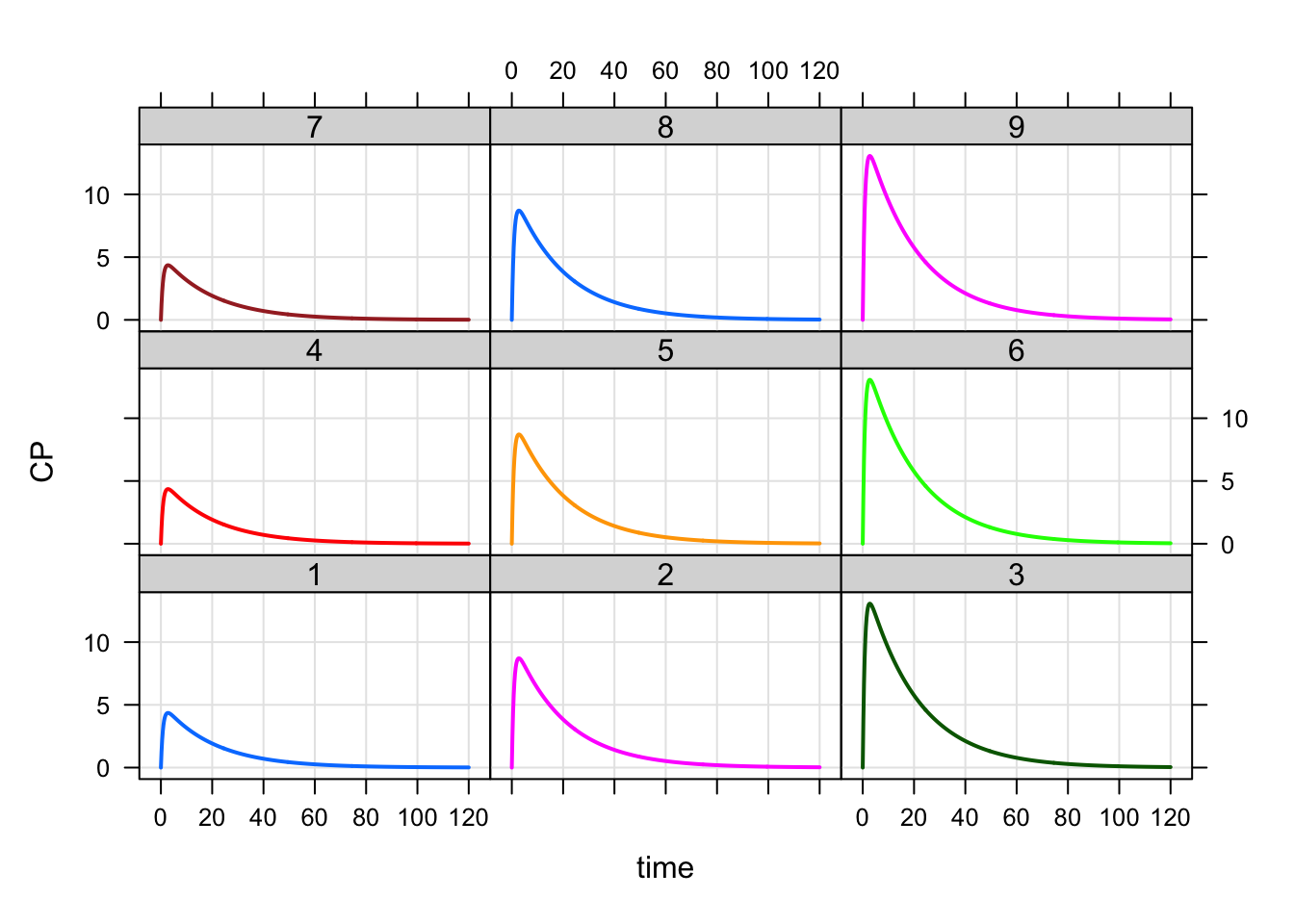
2.2
as_data_set
This function allows you to combine several event objects into a single data sets. An example works best to illustrate.
First, create three event objects. Let’s try one ID at
100 mg, two IDs at 200 mg, and 3 IDs at 300
mg.
e1 <- ev(amt=100, ID=1)
e2 <- ev(amt=200, ID=1:2)
e3 <- ev(amt=300, ID=1:3)
The events are
e1. Events:
. ID time amt cmt evid
. 1 1 0 100 1 1and
e2. Events:
. ID time amt cmt evid
. 1 1 0 200 1 1
. 2 2 0 200 1 1and
e3. Events:
. ID time amt cmt evid
. 1 1 0 300 1 1
. 2 2 0 300 1 1
. 3 3 0 300 1 1When we combine these events with as_data_set we get
data <- as_data_set(e1,e2,e3)
data
. ID time cmt evid amt
. 1 1 0 1 1 100
. 2 2 0 1 1 200
. 3 3 0 1 1 200
. 4 4 0 1 1 300
. 5 5 0 1 1 300
. 6 6 0 1 1 300A nice feature of as_data_set is, unlike
expand.ev and the previous example, we can use complicated
event sequences that are expressed with more than one line in the data
set. For example, consider the case where every ID gets a
250 mg loading dose, and then either get 250 mg q24h, or 120 mg q12h or
500 mg q48h.
load <- function(n) ev(amt=250, ID=1:n)
e1 <- load(1) + ev(amt=250, time=24, ii=24, addl=3, ID=1)
e2 <- load(2) + ev(amt=125, time=24, ii=12, addl=7, ID=1:2)
e3 <- load(3) + ev(amt=500, time=24, ii=48, addl=1, ID=1:3)
Now, e1, e2, and e3 are more
complex
e1. Events:
. ID time amt cmt evid ii addl
. 1 1 0 250 1 1 0 0
. 2 1 24 250 1 1 24 3e3. Events:
. ID time amt cmt evid ii addl
. 1 1 0 250 1 1 0 0
. 4 1 24 500 1 1 48 1
. 2 2 0 250 1 1 0 0
. 5 2 24 500 1 1 48 1
. 3 3 0 250 1 1 0 0
. 6 3 24 500 1 1 48 1But, we can still pull them together in one single data set
data <- as_data_set(e1,e2,e3)
data
. ID time cmt evid amt ii addl
. 1 1 0 1 1 250 0 0
. 2 1 24 1 1 250 24 3
. 3 2 0 1 1 250 0 0
. 4 2 24 1 1 125 12 7
. 5 3 0 1 1 250 0 0
. 6 3 24 1 1 125 12 7
. 7 4 0 1 1 250 0 0
. 8 4 24 1 1 500 48 1
. 9 5 0 1 1 250 0 0
. 10 5 24 1 1 500 48 1
. 11 6 0 1 1 250 0 0
. 12 6 24 1 1 500 48 1An example simulation
set.seed(1112)
mod %>%
  omat(dmat(1,1,1,1)/10) %>%
  data_set(data) %>%
  mrgsim() %>%
  plot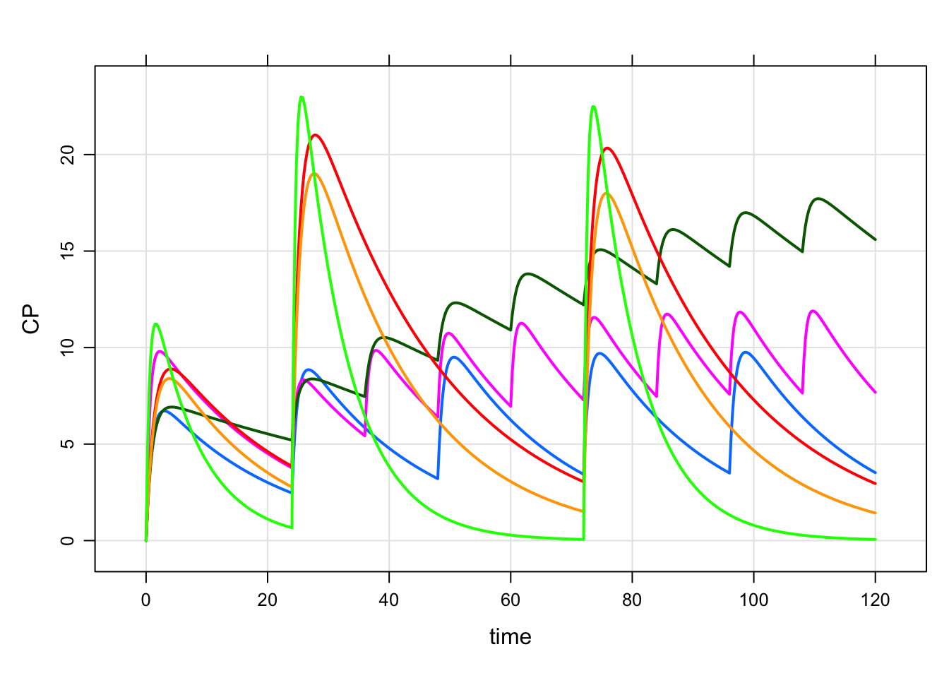
2.3
as.data.frame.ev
Just a quick reminder here that you can easily convert between a
single event object and a data.frame
as.data.frame(e3). ID time amt cmt evid ii addl
. 1 1 0 250 1 1 0 0
. 4 1 24 500 1 1 48 1
. 2 2 0 250 1 1 0 0
. 5 2 24 500 1 1 48 1
. 3 3 0 250 1 1 0 0
. 6 3 24 500 1 1 48 1as.ev(as.data.frame(e3)). Events:
. ID time amt ii addl cmt evid
. 1 1 0 250 0 0 1 1
. 4 1 24 500 48 1 1 1
. 2 2 0 250 0 0 1 1
. 5 2 24 500 48 1 1 1
. 3 3 0 250 0 0 1 1
. 6 3 24 500 48 1 1 1So if you were building up an event object and just wanted to use it
as a data_set or as a building block for a
data_set, just coerce with as.data.frame.
2.4
assign_ev
This function assigns an intervention in the form of an event object
to individuals in an idata_set according to a grouping
column.
To illustrate, make a simple idata_set
set.seed(8)
idata <- data_frame(ID=sample(1:6), arm=c(1,2,2,3,3,3))
idata
. # A tibble: 6 × 2
. ID arm
. <int> <dbl>
. 1 4 1
. 2 2 2
. 3 3 2
. 4 6 3
. 5 5 3
. 6 1 3Here, we have 6 IDs, one in arm 1, two in arm 2, three
in arm 3. Let’s take the events from the previous example and assign
them to the different arms.
e1 <- ev(amt=250) + ev(amt=250, time=24, ii=24, addl=3)
e2 <- ev(amt=250) + ev(amt=125, time=24, ii=12, addl=7)
e3 <- ev(amt=250) + ev(amt=500, time=24, ii=48, addl=1)
assign_ev(list(e3,e2,e1),idata,"arm")
. time amt cmt evid ii addl ID
. 1 0 250 1 1 0 0 4
. 2 24 500 1 1 48 1 4
. 3 0 250 1 1 0 0 2
. 4 24 125 1 1 12 7 2
. 5 0 250 1 1 0 0 3
. 6 24 125 1 1 12 7 3
. 7 0 250 1 1 0 0 6
. 8 24 250 1 1 24 3 6
. 9 0 250 1 1 0 0 5
. 10 24 250 1 1 24 3 5
. 11 0 250 1 1 0 0 1
. 12 24 250 1 1 24 3 1Please look carefully at the input (idata and
list(e3,e2,e1)); I have mixed it up a bit here to try to
illustrate how things are assigned.
2.5
ev_days
This is a recently-added function (hint: you might need to install the latest version from GitHub to use this) that lets you schedule certain events on certain days of the week, repeating in a weekly cycle.
For example, to schedule 250 mg doses every Monday, Wednesday, and Friday for a month, you can do
data <- ev_days(ev(amt=250, ID=1), days="m,w,f", addl=3)
data
. ID time amt cmt evid ii addl
. 1 1 0 250 1 1 168 3
. 2 1 48 250 1 1 168 3
. 3 1 96 250 1 1 168 3mod %>% mrgsim(data=data,end=168*4) %>% plot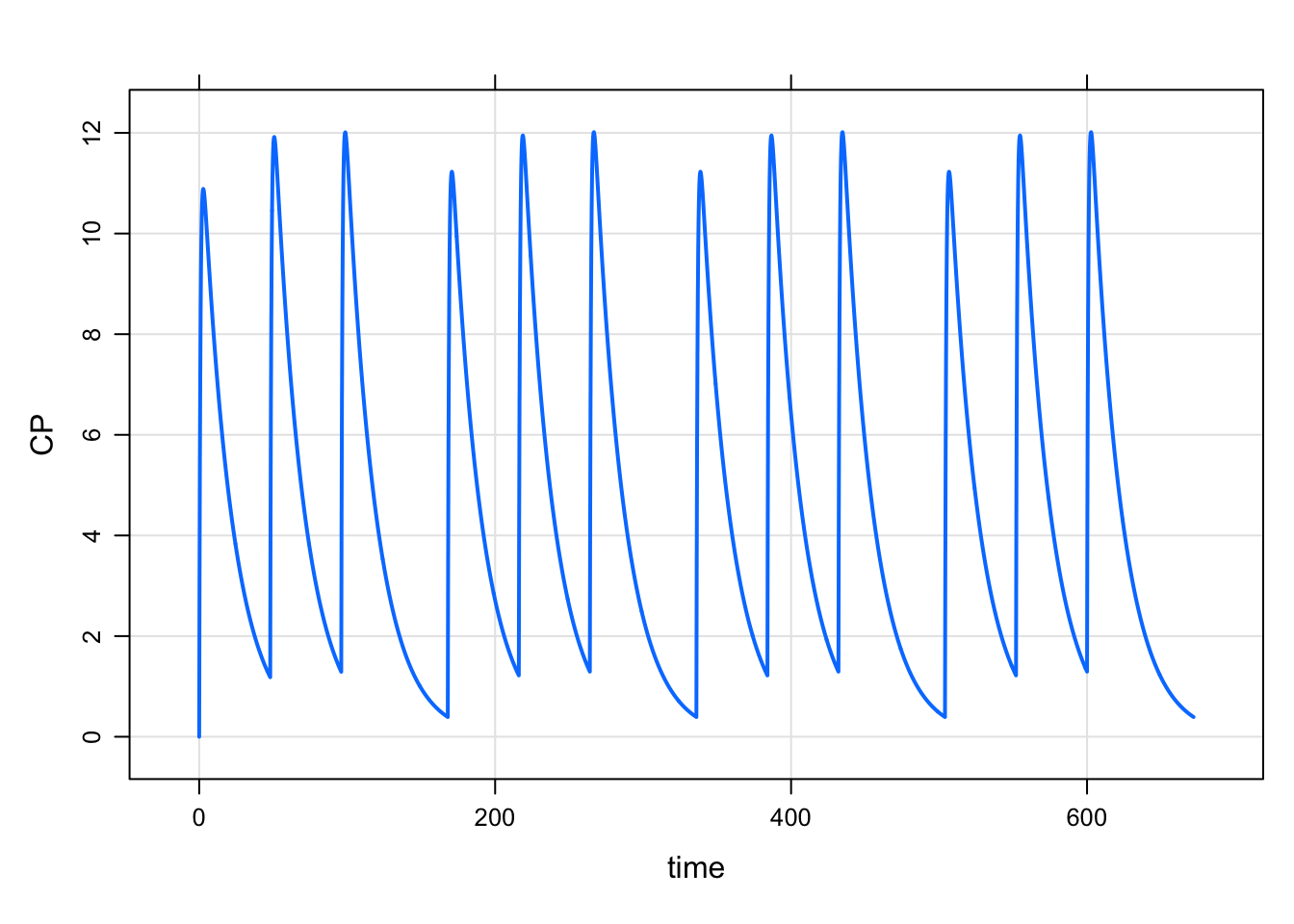
Or, you can do 100 mg doses on Monday, Wednesday, Friday, and 50 mg doses on Tuesday, Thursday, with drug holiday on weekends
e1 <- ev(amt=100,ID=1)
e2 <- ev(amt=50,ID=1)
data <- ev_days(m=e1,w=e1,f=e1,t=e2,th=e2,addl=3)
data
. ID time amt cmt evid ii addl
. 1 1 0 100 1 1 168 3
. 2 1 24 50 1 1 168 3
. 3 1 48 100 1 1 168 3
. 4 1 72 50 1 1 168 3
. 5 1 96 100 1 1 168 3And simulate
mod %>% mrgsim(data=data,end=168*4) %>% plot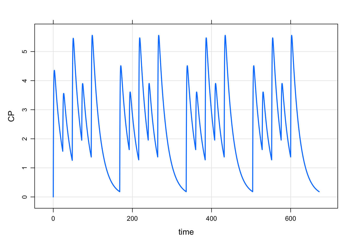
The same thing can be accomplished like this
a <- ev_days(e1,days="m,w,f",addl=3)
b <- ev_days(e2,days="t,th",addl=3)

c(as.ev(a),as.ev(b))
. Events:
. ID time amt ii addl cmt evid
. 1 1 0 100 168 3 1 1
. 4 1 24 50 168 3 1 1
. 2 1 48 100 168 3 1 1
. 5 1 72 50 168 3 1 1
. 3 1 96 100 168 3 1 1data.frame to use as a data_set.
3 Filter input data set inline
Remember, when you pass in your input data set via
data_set, you can filter in line:
data <- expand.ev(amt=c(100,200,300))
mod %>% data_set(data, amt==300) %>% Req(GUT,CP) %>% mrgsim
. Model: housemodel
. Dim: 482 x 4
. Time: 0 to 120
. ID: 1
. ID time GUT CP
. 1: 3 0.00 0.00 0.000
. 2: 3 0.00 300.00 0.000
. 3: 3 0.25 222.25 3.862
. 4: 3 0.50 164.64 6.676
. 5: 3 0.75 121.97 8.712
. 6: 3 1.00 90.36 10.174
. 7: 3 1.25 66.94 11.211
. 8: 3 1.50 49.59 11.934mrgsolve: mrgsolve.github.io | metrum research group: metrumrg.com